Global Temerature: Climate Change?
Let the data tell the truth.
Introduction
With the recent news that global high temperatures are breaking records and being annoyed by the Democrats fighting the Republicans whether this or is this or is not caused by human factors, I decided to make my own decision based on the facts available.
Since temperature data is available only for a couple of hundred of years, it becomes a bit harder to make a 100% confident statement supporting or negating human caused climate warning. We can look much further in the past using data derived from ancient ice samples, so that alleviates some of the concern around having relatively limited hard temperature data, but we can still reach a valid, data-driven conclusion.
Let’s see what the data say.
Global Surface Temperatures: The Data
The data comes from the NASA GISS Surface Temperature Analysis (GISTEMP v4). The datasets are tables of global and hemispheric monthly means and zonal annual means. They combine land-surface, air and sea-surface water temperature anomalies (Land-Ocean Temperature Index, L-OTI). The values in the tables are deviations from the corresponding 1951-1980 means.
There’s also more detail and answers to commonly asked in questions in their FAQ.
- Global-mean monthly, seasonal, and annual means, 1880-present, updated through most recent month [Ggobal]
- Northern Hemisphere-mean monthly, seasonal, and annual means, 1880-present, updated through most recent month [nh]
- Southern Hemisphere-mean monthly, seasonal, and annual means, 1880-present, updated through most recent month [sh]
- Zonal annual means, 1880-present, updated through most recent complete year [zonann]
Citation: GISTEMP Team, 2023: GISS Surface Temperature Analysis (GISTEMP), version 4. NASA Goddard Institute for Space Studies. Dataset accessed 2023-07-09 at https://data.giss.nasa.gov/gistemp/
The focus of this document uses the Global data.
Get Data
global_temps <- readr::read_csv('https://raw.githubusercontent.com/rfordatascience/tidytuesday/master/data/2023/2023-07-11/global_temps.csv')
nh_temps <- readr::read_csv('https://raw.githubusercontent.com/rfordatascience/tidytuesday/master/data/2023/2023-07-11/nh_temps.csv')
sh_temps <- readr::read_csv('https://raw.githubusercontent.com/rfordatascience/tidytuesday/master/data/2023/2023-07-11/sh_temps.csv')
zonann_temps <- readr::read_csv('https://raw.githubusercontent.com/rfordatascience/tidytuesday/master/data/2023/2023-07-11/zonann_temps.csv')

#Save raw data
write_csv(global_temps, "data/global_temps.csv")
write_csv(global_temps, "data/nh_temps.csv")
write_csv(global_temps, "data/sh_temps.csv")
write_csv(global_temps, "data/zonann_temps.csv")
Data Dictionary
# https://github.com/rfordatascience/tidytuesday/blob/master/data/2023/2023-07-11/readme.md
global_temps_dict <- read.delim("clipboard")
nh_temps_dict <- read.delim("clipboard")
sh_temps_dict <- read.delim("clipboard")
zonann_temps_dict <- read.delim("clipboard")

write_csv(global_temps_dict, "data/global_temps_dict.csv")
write_csv(nh_temps_dict, "data/nh_temps_dict.csv")
write_csv(sh_temps_dict, "data/sh_temps_dict.csv")
write_csv(zonann_temps_dict, "data/zonann_temps_dict.csv")
g1 <- global_temps_dict %>% gt() %>%
cols_label(variable = md('**Variable**'), class = md('**Class**'), description = md('**Description**')) %>%
tab_header(title = md("**Temperature Data Dictionary**"), subtitle = "Global, Norther & Southern Hemispheres") %>%
opt_stylize(style=3)
g4 <- zonann_temps_dict %>% gt() %>%
cols_label(variable = md('**Variable**'), class = md('**Class**'), description = md('**Description**')) %>%
tab_header(title = md("**Temperature Data Dictionary**"), subtitle = "Zonal Data") %>%
opt_stylize(style=3)listed_tables <- list(g1, g4)
gt_two_column_layout(listed_tables)| Temperature Data Dictionary | ||
| Global, Norther & Southern Hemispheres | ||
| Variable | Class | Description |
|---|---|---|
| Year | double | Year |
| Jan | double | January |
| Feb | double | February |
| Mar | double | March |
| Apr | double | April |
| May | double | May |
| Jun | double | June |
| Jul | double | July |
| Aug | double | August |
| Sep | double | September |
| Oct | double | October |
| Nov | double | November |
| Dec | double | December |
| J-D | double | January-December |
| D-N | double | Decemeber-November |
| DJF | double | December-January-February |
| MAM | double | March-April-May |
| JJA | double | June-July-August |
| SON | double | September-October-November |
| Temperature Data Dictionary | ||
| Zonal Data | ||
| Variable | Class | Description |
|---|---|---|
| Year | double | Year |
| Glob | double | Global |
| NHem | double | Northern Hemisphere |
| SHem | double | Southern Hemisphere |
| 24N-90N | double | 24N-90N lattitude |
| 24S-24N | double | 24S-24N lattitude |
| 90S-24S | double | 90S-24S lattitude |
| 64N-90N | double | 64N-90N lattitude |
| 44N-64N | double | 44N-64N lattitude |
| 24N-44N | double | 24N-44N lattitude |
| EQU-24N | double | EQU-24N lattitude |
| 24S-EQU | double | 24S-EQU lattitude |
| 44S-24S | double | 44S-24S lattitude |
| 64S-44S | double | 64S-44S lattitude |
| 90S-64S | double | 90S-64S lattitude |
A quick look informed me that there are 2 years with incomplete data: 1880 and 2023 (of course since it is only August). This missing data was consistent across the 4 data sets so I have simply removed them.
global_temps %>% filter(if_any(.cols = everything(), .fns = is.na)) # A tibble: 2 × 19
Year Jan Feb Mar Apr May Jun Jul Aug Sep Oct Nov Dec
<dbl> <dbl> <dbl> <dbl> <dbl> <dbl> <dbl> <dbl> <dbl> <dbl> <dbl> <dbl> <dbl>
1 1880 -0.19 -0.25 -0.09 -0.17 -0.1 -0.21 -0.18 -0.11 -0.15 -0.24 -0.22 -0.18
2 2023 0.87 0.98 1.21 1 0.94 NA NA NA NA NA NA NA
# ℹ 6 more variables: `J-D` <dbl>, `D-N` <dbl>, DJF <dbl>, MAM <dbl>,
# JJA <dbl>, SON <dbl>The data is provided in wide format. Will transform into long format.
Dropping the seasonal data and only retaining the monthly data. Then reshape it into three columns: Year, Month, and Change in temperature. Also convert from C to F (1° C = 1.8° F)
global_temps_reshaped <- global_temps %>% select(Year:Dec) %>%
  pivot_longer(Jan:Dec, names_to = "Month", values_to = "Change")
global_temps_reshaped <- global_temps_reshaped %>% mutate(Change = 1.8 * Change)
head(global_temps_reshaped)
# A tibble: 6 × 3
Year Month Change
<dbl> <chr> <dbl>
1 1881 Jan -0.36
2 1881 Feb -0.27
3 1881 Mar 0.054
4 1881 Apr 0.09
5 1881 May 0.09
6 1881 Jun -0.342Change the class for Month and Year.
global_temps_reshaped$Month <- factor(global_temps_reshaped$Month, levels = month.abb)
global_temps_reshaped$Year <- as.integer(global_temps_reshaped$Year)
Visualizations
Colored Line Plot
global_temps$Annual_Mean <- rowMeans(global_temps[, 2:13], na.rm = TRUE)

ggplot(global_temps, aes(x = Year, y = Annual_Mean, color = Annual_Mean)) +
  geom_line(linewidth = 2, lineend = "round") +
  scale_color_viridis_c(option = "magma", direction = 1) +
  scale_x_continuous(breaks = seq(1880, 2020, 20)) +
  labs(x = "Year", y = "Annual Mean Temperature Anomaly (°F)",
       title = "Global Surface Temperature Trend",
       subtitle = "Annual Mean Temperature Anomalies",
       caption = "Source: GISTEMP Team, 2023: GISS Surface Temperature Analysis") +
  theme_minimal() +
  theme(plot.title = element_text(size = 24, face = "bold", hjust = 0.5),
        plot.subtitle = element_text(size = 14, hjust = 0.5),
        plot.caption = element_text(size = 9, hjust = 0),
        axis.text.x = element_text(size = 12),
        axis.text.y = element_text(size = 12),
        legend.position = "none",
        panel.grid.major.x = element_blank(),
        panel.grid.minor.x = element_blank(),
        panel.grid.major.y = element_line(color = "gray90"),
        panel.grid.minor.y = element_line(color = "gray95"),
        panel.background = element_rect(fill = "gray98"),
        plot.margin = margin(20, 20, 20, 20))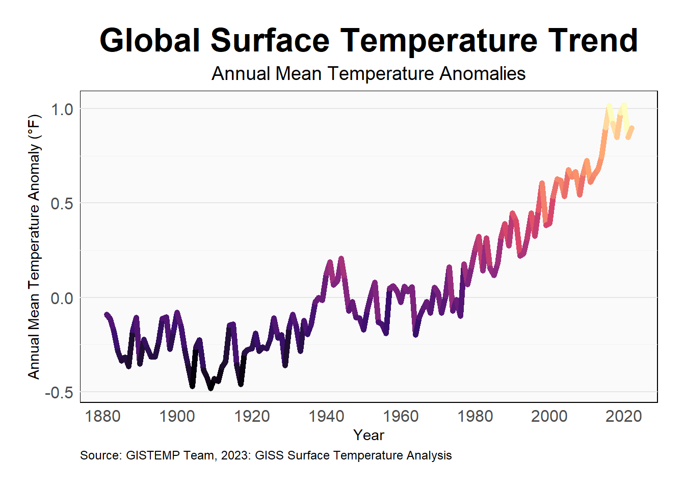
Animated Bar Plot
animate1 <- global_temps_reshaped %>%
ggplot(aes(Month, Change, fill = Change)) + geom_col() +
scale_fill_viridis(option = "turbo", name = "\U0394 T (\U00B0 F)") +
ylim(-2.0, 2.7) + theme_classic(12) +
labs(x = "", y = "\U0394 Temperature (\U00B0 F)") +
labs(title = "Global Deviations in Temperature",
subtitle = "Year: <b>{frame_time}</b>",
caption = "<b>Data from: NASA GISTEMP</b><i><span style = 'font-size:11pt;'>https://www.data.giss.nasa.gov/gistemp/</span></i> <br>
<i><span style = 'font-size:10pt;color:darkgrey'>Worldwide scientific bodies have used 1.5 \U00B0 C as the standard measure.<br>This has been converted to \U00B0 F for this document.</span></i>") +
theme(plot.title = element_markdown(color = "steelblue", hjust = 0.5, size = 16),
plot.caption = element_markdown(size = 12),
plot.subtitle = element_markdown(color = "steelblue", size = 14),
axis.title.y = element_markdown(size = 10),
axis.title.x = element_markdown(size = 10),
legend.text = element_markdown(size = 10),
legend.title = element_markdown(size=12)) +
transition_time(Year) + ease_aes('cubic-in-out')animate(animate1, duration = 40, fps = 20)
anim_save("temperature_bar.gif", animation = last_animation(), path = "animation/")
Polar Coordinant Animated Plot
bg_col <- "grey30"
highlight_col <- "#d6604d"
text_col <- "white"

# text
title <- "Global Surface Temperatures"
st <- "The GISS Surface Temperature Analysis is an estimate of global surface temperature change,
combining land-surface, air and sea-surface water temperature anomalies. Here, values relate to
deviations from the 1951-1980 average."

cap <- "**Data**: NASA GISS Surface Temperature Analysis"

# animate
  animate_polar <- plot_data %>%
    ggplot(aes(x = Month, y = Change, group = Year, color = Change)) +
    geom_line() +
    labs(x = "", y = NULL, title = title, subtitle = st, caption = cap, tag = "Year: <b>{frame_time}</b>") +
    scale_color_distiller(limits = c(-2.0, 2.7), palette = "RdYlBu") +
    scale_x_discrete(expand = c(0,0), breaks = month.abb, drop = FALSE) +
    scale_y_continuous(limits = c(-2.0, 2.7)) +
    guides(color = guide_colorbar(title = "Temperature deviation (°F)",
                                  title.position = "top", title.hjust = 0.5,
                                  barwidth = 15, barheight = 0.7)) +
    coord_polar() +
    theme_minimal(base_size = 18, base_family = "Commissioner") + # size was 24
    theme(legend.position = c(0.5, -0.05), #-.1
          legend.direction = "horizontal",
          legend.text = element_text(color = text_col),
          legend.title = element_text(color = highlight_col),
          plot.tag.position = c(0.46, 0.75),
          plot.tag = element_markdown(family = "Commissioner",
                                            color = highlight_col,
                                            size = 20, # was 36
                                            hjust = 0.3, #lineheight = 0.4,#hjust was .2, .1 seemed lower
                                            vjust = -0.62,
                                            #linetype = 1, box.color = "#1F618D", fill = "#1F618D",
                                            padding = margin(2,2,2,8),
                                            margin = margin(t = 6, b = 10)),

          axis.text.x = element_text(color = text_col),
          axis.text.y = element_blank(),
          panel.grid.major.x = element_line(linewidth = 0.3, color = alpha(text_col, 0.4)),
          panel.grid.major.y = element_blank(),
          plot.background = element_rect(fill = bg_col, color = bg_col),
          panel.background = element_rect(fill = bg_col, color = bg_col),
          plot.margin = margin(10, 15, 10, 10),
          plot.title = element_markdown(family = "Fraunces",
                                        color = highlight_col, face = "bold",
                                        hjust = 0, size = 30, #size was 40
                                        margin = margin(t = 20)),
          plot.subtitle = element_textbox_simple(family = "Commissioner",
                                                 color = text_col,
                                                 lineheight = 0.5,
                                                 margin = margin(t = 20, b = 20)), # b=30
          plot.caption = element_markdown(family = "Commissioner",
                                          color = "grey",
                                          hjust =  0, #lineheight = 0.5,
                                          margin = margin(t = 40))) +
    transition_time(Year) + shadow_mark()
Conclusion
The world is experiencing record-breaking heat in 2023. The world’s average daily temperature soared to highs unseen in modern records kept by two climate agencies in the US and Europe¹. The records are based on data that only goes back to the mid-20th century, but they are almost certainly the warmest the planet has seen over a much longer time period, probably going back at least 100,000 years.
The world experienced its warmest June on record by a substantial margin. Ocean heat has been off the charts, with surface temperatures reaching record levels for June 2023. Parts of the North Atlantic have seen an unprecedented marine heat wave, with temperatures up to 9 degrees Fahrenheit hotter than usual. And in Antarctica, where temperatures are running well-above average for this time of year, sea ice plunged to record low levels.
The warmest day on record for the entire planet was July 6, 2023, when the highest global average temperature was recorded at 62.74 °F). The month of July 2023 was also the hottest month on record globally.
These are just some of the many heat records that have been broken in 2023. It is a clear indication that global warming is having a significant impact on our planet.
Above should not be news to anyone. The number of heat records worklwide is something none have us have witnessed in our lifetime.
The numbers prove beyond a reasonable doubt that indeed the planet is warming. This document does not investigate the reason for this - it is an argument that is very partisan and I am not here to start an argument. (OK, be honest, the human species is at least partially to blame - if not more, for this warming phenomenon.)
So what might happen as a result of global warming?
- Coral reefs face almost complete die-off
- ‘Unheard-of’ storms become more common
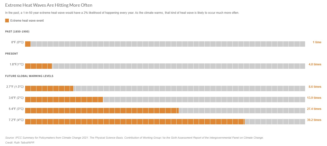 - Melting ice leads to flooded cities - More than 4 million people in the U.S. are at risk along coastlines, where higher sea levels would cause bigger storm surges and higher high tides.
There is sufficient evidence that climate change is a real problem. Anyone that ignores the facts and relies in social media and other outlets are simply fooling themselves. Some facts are simply too obvious to allow those that still think the world is flat to drive our plans for the future so that our children’s children have a suitably safe world in which to thrive.