Python Streamlit Example
Introduction
While I much prefer R and Shiny to publish solutions, I do not reject Python platforms for publishing data science projects. Below, I have used Pycaret and Steamlit to build a blended machine learning model and published the application on Streamlit.
What I learned is Pycaret is an easy to use and powerful automated machine learning Python module. Also, Streamlit is very easy to use and you can publish your application for free just as you can a Shiny application.
Will I stop using R and Shiny instead of Python alternatives? No, unless the business case requires me to do so.
import numpy as np
import pandas as pd
from pycaret.regression import *

dataset = pd.read_csv("insurance.csv")
dataset.head()
Get Data
| Insurance Data | ||||||
| age | sex | bmi | children | smoker | region | charges |
|---|---|---|---|---|---|---|
| 19 | female | 27.900 | 0 | yes | southwest | 16884.924 |
| 18 | male | 33.770 | 1 | no | southeast | 1725.552 |
| 28 | male | 33.000 | 3 | no | southeast | 4449.462 |
| 33 | male | 22.705 | 0 | no | northwest | 21984.471 |
| 32 | male | 28.880 | 0 | no | northwest | 3866.855 |
data = dataset.sample(frac=0.9, random_state=786)
data_unseen = dataset.drop(data.index)

data.reset_index(drop=True, inplace=True)
data_unseen.reset_index(drop=True, inplace=True)

print('Data for Modeling: ' + str(data.shape))
print('Unseen Data For Predictions: ' + str(data_unseen.shape))
Data for Modeling: (1204, 7) Unseen Data For Predictions: (134, 7)
s = setup(data, target = 'charges', session_id = 123,
           normalize = True, silent = True,
           polynomial_features = True, trigonometry_features = True,
           feature_interaction=True,
           bin_numeric_features= ['age', 'bmi'])
Pycaret Feature Engineering and Selection
read.delim("texttable2.txt", sep = "\t") %>%as_tibble() %>%  select(Description, Value) %>%
  gt() %>% tab_header(title = md("**Pycaret Data Features**")) %>%
tab_style(style = list(cell_fill(color="green")), locations = cells_body(columns = c(Description, Value), rows = Value == "True"))| Pycaret Data Features | |
| Description | Value |
|---|---|
| session_id | 123 |
| Target | charges |
| Original Data | (1204, 7) |
| Missing Values | False |
| Numeric Features | 2 |
| Categorical Features | 4 |
| Ordinal Features | False |
| High Cardinality Features | False |
| High Cardinality Method | None |
| Transformed Train Set | (842, 58) |
| Transformed Test Set | (362, 58) |
| Shuffle Train-Test | True |
| Stratify Train-Test | False |
| Fold Generator | KFold |
| Fold Number | 10 |
| CPU Jobs | -1 |
| Use GPU | False |
| Log Experiment | False |
| Experiment Name | reg-default-name |
| USI | da99 |
| Imputation Type | simple |
| Iterative Imputation Iteration | None |
| Numeric Imputer | mean |
| Iterative Imputation Numeric Model | None |
| Categorical Imputer | constant |
| Iterative Imputation Categorical Model | None |
| Unknown Categoricals Handling | least_frequent |
| Normalize | True |
| Normalize Method | zscore |
| Transformation | False |
| Transformation Method | None |
| PCA | False |
| PCA Method | None |
| PCA Components | None |
| Ignore Low Variance | False |
| Combine Rare Levels | False |
| Rare Level Threshold | None |
| Numeric Binning | True |
| Remove Outliers | False |
| Outliers Threshold | None |
| Remove Multicollinearity | False |
| Multicollinearity Threshold | None |
| Remove Perfect Collinearity | True |
| Clustering | False |
| Clustering Iteration | None |
| Polynomial Features | True |
| Polynomial Degree | 2 |
| Trignometry Features | True |
| Polynomial Threshold | 0.100000 |
| Group Features | False |
| Feature Selection | False |
| Feature Selection Method | classic |
| Features Selection Threshold | None |
| Feature Interaction | True |
| Feature Ratio | False |
| Interaction Threshold | 0.010000 |
| Transform Target | False |
| Transform Target Method | box-cox |
Modeling
compare_models(fold=20, n_select=10)tbl3 <- read.delim("texttable3.txt", sep = "\t") %>%as_tibble()
min_mse = min(tbl3$MSE)
max_r2 = max(tbl3$R2)
min_rmse = min(tbl3$RMSE)
min_mae = min(tbl3$MAE)
min_rmsle = min(tbl3$RMSLE)
min_mape = min(tbl3$MAPE)
tbl3 <- tbl3 %>% gt() %>% tab_header(title = md("**Model Performance Comparison**")) %>%
tab_style(style = list(cell_fill(color = "green")), locations = cells_body(columns = c(MSE), rows = MSE == min_mse)) %>%
tab_style(style = list(cell_fill(color = "green")), locations = cells_body(columns = c(MAE), rows = MAE == min_mae)) %>%
tab_style(style = list(cell_fill(color = "green")), locations = cells_body(columns = c(R2), rows = R2 == max_r2)) %>%
tab_style(style = list(cell_fill(color = "green")), locations = cells_body(columns = c(RMSE), rows = RMSE == min_rmse)) %>%
tab_style(style = list(cell_fill(color = "green")), locations = cells_body(columns = c(RMSLE), rows = RMSLE == min_rmsle)) %>%
tab_style(style = list(cell_fill(color = "green")), locations = cells_body(columns = c(MAPE), rows = MAPE == min_mape))
tbl3| Model Performance Comparison | |||||||
| Model | MAE | MSE | RMSE | R2 | RMSLE | MAPE | TT..Sec. |
|---|---|---|---|---|---|---|---|
| Lasso Least Angle Regression | 2732.596 | 2.104770e+07 | 4523.254 | 8.42300e-01 | 0.4220 | 0.3214 | 0.0145 |
| Ridge Regression | 2728.936 | 2.108289e+07 | 4519.783 | 8.42000e-01 | 0.4083 | 0.2998 | 0.0115 |
| Bayesian Ridge | 2735.247 | 2.112505e+07 | 4526.634 | 8.41800e-01 | 0.4085 | 0.3008 | 0.0160 |
| Linear Regression | 2727.752 | 2.105203e+07 | 4505.568 | 8.41600e-01 | 0.4104 | 0.2984 | 1.1405 |
| Lasso Regression | 2716.907 | 2.109591e+07 | 4515.338 | 8.41600e-01 | 0.4089 | 0.2972 | 0.0140 |
| Gradient Boosting Regressor | 2553.426 | 2.117309e+07 | 4486.413 | 8.40600e-01 | 0.4306 | 0.3055 | 0.0560 |
| Orthogonal Matching Pursuit | 2853.320 | 2.246594e+07 | 4695.386 | 8.34400e-01 | 0.4432 | 0.3401 | 0.0105 |
| Huber Regressor | 1756.587 | 2.263832e+07 | 4684.403 | 8.31900e-01 | 0.3460 | 0.0731 | 0.0465 |
| Passive Aggressive Regressor | 1741.354 | 2.281087e+07 | 4705.221 | 8.30900e-01 | 0.3474 | 0.0709 | 0.0745 |
| Random Forest Regressor | 2637.197 | 2.274487e+07 | 4651.607 | 8.26800e-01 | 0.4543 | 0.3193 | 0.2225 |
| Light Gradient Boosting Machine | 2862.800 | 2.326736e+07 | 4718.931 | 8.25300e-01 | 0.5139 | 0.3609 | 0.0310 |
| Extra Trees Regressor | 2568.497 | 2.493545e+07 | 4872.980 | 8.09400e-01 | 0.4511 | 0.2984 | 0.2060 |
| K Neighbors Regressor | 3349.147 | 3.449971e+07 | 5815.685 | 7.47600e-01 | 0.4683 | 0.3145 | 0.0390 |
| AdaBoost Regressor | 5023.447 | 3.325294e+07 | 5720.854 | 7.47300e-01 | 0.7227 | 0.9520 | 0.0180 |
| Decision Tree Regressor | 2963.674 | 3.860766e+07 | 6095.674 | 7.09000e-01 | 0.5118 | 0.3331 | 0.0115 |
| Elastic Net | 6242.648 | 6.143278e+07 | 7808.173 | 5.71400e-01 | 0.7065 | 0.8848 | 0.0125 |
| Dummy Regressor | 9409.356 | 1.518491e+08 | 12221.629 | -2.93000e-02 | 1.0215 | 1.5963 | 0.0095 |
| Least Angle Regression | 15534816.771 | 7.669493e+15 | 27427002.595 | -4.84973e+07 | 2.5624 | 3122.1669 | 0.0145 |
Cross Validation
Ridge Regression
ridge=create_model("ridge", fold=10)read.delim("texttable4.txt", sep = "\t") %>%as_tibble() %>%
gt() %>% tab_header(title = md("**Ridge Model Selected**"),
subtitle = md("Ridge model selected after running many iterations.")) %>%
gt_highlight_rows(rows = 11, font_weight = "normal")| Ridge Model Selected | ||||||
| Ridge model selected after running many iterations. | ||||||
| Fold | MAE | MSE | RMSE | R2 | RMSLE | MAPE |
|---|---|---|---|---|---|---|
| 0 | 2644.4497 | 17458422 | 4178.3276 | 0.8888 | 0.3994 | 0.2997 |
| 1 | 2396.6917 | 13792027 | 3713.7617 | 0.9271 | 0.3248 | 0.2947 |
| 2 | 2661.2834 | 16095249 | 4011.8884 | 0.8754 | 0.3945 | 0.3242 |
| 3 | 2803.0896 | 24090658 | 4908.2236 | 0.7923 | 0.4632 | 0.2866 |
| 4 | 3306.9434 | 32729668 | 5720.9849 | 0.7929 | 0.4599 | 0.2634 |
| 5 | 2740.3174 | 20716682 | 4551.5581 | 0.8559 | 0.4226 | 0.3347 |
| 6 | 2968.8784 | 20332018 | 4509.1040 | 0.8883 | 0.3812 | 0.3050 |
| 7 | 2732.5020 | 23839016 | 4882.5215 | 0.7771 | 0.4448 | 0.3143 |
| 8 | 2188.8196 | 12012671 | 3465.9299 | 0.9407 | 0.3604 | 0.3137 |
| 9 | 2865.0833 | 28998558 | 5385.0308 | 0.7451 | 0.4542 | 0.2699 |
| Mean | 2730.8058 | 21006497 | 4532.7331 | 0.8483 | 0.4105 | 0.3006 |
| Std | 288.0337 | 6237200 | 678.8429 | 0.0638 | 0.0442 | 0.0216 |
tuned_ridge=tune_model(ridge)read.delim("texttable5.txt", sep = "\t") %>%as_tibble() %>%
gt() %>% tab_header(title = md("**Tuned Ridge Model Selected**")) %>%
gt_highlight_rows(rows = 11, font_weight = "normal")| Tuned Ridge Model Selected | ||||||
| Fold | MAE | MSE | RMSE | R2 | RMSLE | MAPE |
|---|---|---|---|---|---|---|
| 0 | 2638.0696 | 17719748 | 4209.4829 | 0.8871 | 0.3964 | 0.2979 |
| 1 | 2464.8701 | 14317923 | 3783.9031 | 0.9243 | 0.3290 | 0.2996 |
| 2 | 2700.9890 | 16758014 | 4093.6553 | 0.8702 | 0.3928 | 0.3202 |
| 3 | 2821.5364 | 24214992 | 4920.8730 | 0.7913 | 0.4737 | 0.2893 |
| 4 | 3210.9170 | 31561262 | 5617.9409 | 0.8003 | 0.4497 | 0.2572 |
| 5 | 2770.4917 | 20765924 | 4556.9644 | 0.8556 | 0.4207 | 0.3365 |
| 6 | 3000.1746 | 20701708 | 4549.9131 | 0.8862 | 0.3835 | 0.3088 |
| 7 | 2752.6213 | 23780156 | 4876.4902 | 0.7776 | 0.4478 | 0.3218 |
| 8 | 2220.6887 | 12428095 | 3525.3503 | 0.9386 | 0.3579 | 0.3129 |
| 9 | 2808.0850 | 28607576 | 5348.6050 | 0.7485 | 0.4481 | 0.2645 |
| Mean | 2738.8443 | 21085540 | 4548.3178 | 0.8480 | 0.4100 | 0.3009 |
| Std | 256.7305 | 5783024 | 631.1453 | 0.0616 | 0.0437 | 0.0238 |
plot_model(ridge, plot="residuals")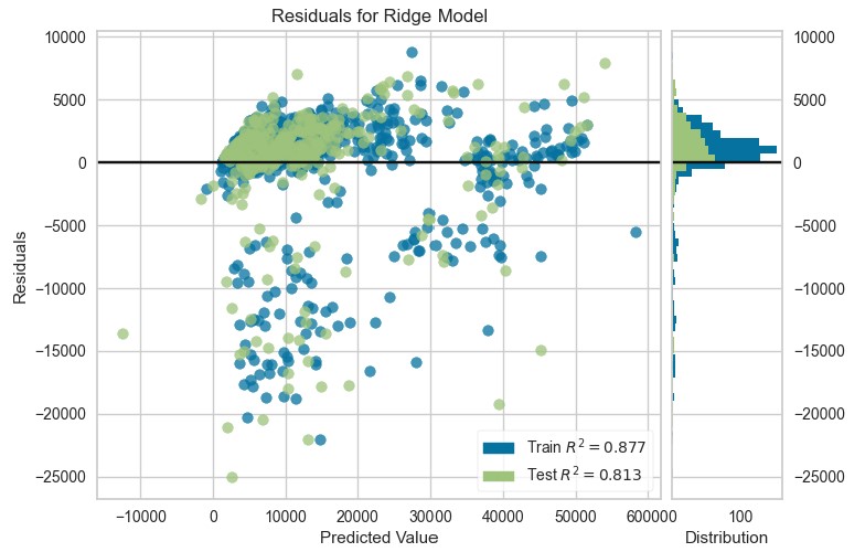
plot_model(ridge, plot="error")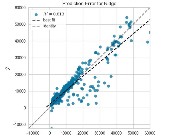
Lasso Regression
lr = tune_model(create_model("lr", fold=10))read.delim("texttable6.txt", sep = "\t") %>%as_tibble() %>%
gt() %>% tab_header(title = md("**Tuned Lasso Regression**")) %>%
gt_highlight_rows(rows = 11, font_weight = "normal")| Tuned Lasso Regression | ||||||
| Fold | MAE | MSE | RMSE | R2 | RMSLE | MAPE |
|---|---|---|---|---|---|---|
| 0 | 2653.5310 | 17379078 | 4168.822 | 0.8893 | 0.4169 | 0.3015 |
| 1 | 2298.0444 | 11653536 | 3413.727 | 0.9384 | 0.3191 | 0.2889 |
| 2 | 2662.1392 | 15827221 | 3978.344 | 0.8774 | 0.3982 | 0.3281 |
| 3 | 2814.8789 | 24249588 | 4924.387 | 0.7910 | 0.4516 | 0.2794 |
| 4 | 3427.0925 | 34247512 | 5852.137 | 0.7833 | 0.4756 | 0.2746 |
| 5 | 2737.7075 | 20867530 | 4568.099 | 0.8548 | 0.4244 | 0.3338 |
| 6 | 2925.0276 | 20040368 | 4476.647 | 0.8899 | 0.3787 | 0.2985 |
| 7 | 2741.3254 | 24315856 | 4931.111 | 0.7726 | 0.4553 | 0.3135 |
| 8 | 2193.4858 | 11721570 | 3423.678 | 0.9421 | 0.3647 | 0.3170 |
| 9 | 2885.1521 | 29481826 | 5429.717 | 0.7408 | 0.4596 | 0.2691 |
| Mean | 2733.8385 | 20978409 | 4516.667 | 0.8480 | 0.4144 | 0.3004 |
| Std | 322.5177 | 6951552 | 760.347 | 0.0678 | 0.0470 | 0.0214 |
Gradient Boosting Regression Model
gbr=tune_model(create_model("gbr", fold=10))read.delim("texttable7.txt", sep = "\t") %>%as_tibble() %>%
gt() %>% tab_header(title = md("**Gradient Boosting Regression Model**")) %>%
gt_highlight_rows(rows = 11, font_weight = "normal")| Gradient Boosting Regression Model | ||||||
| Fold | MAE | MSE | RMSE | R2 | RMSLE | MAPE |
|---|---|---|---|---|---|---|
| 0 | 3183.1979 | 24621592 | 4962.0149 | 0.8431 | 0.5329 | 0.4181 |
| 1 | 2398.5225 | 11020166 | 3319.6636 | 0.9417 | 0.6118 | 0.3837 |
| 2 | 2857.3699 | 20660735 | 4545.4082 | 0.8400 | 0.4839 | 0.3977 |
| 3 | 3906.2212 | 41214576 | 6419.8579 | 0.6447 | 0.7550 | 0.4224 |
| 4 | 3625.8021 | 37865167 | 6153.4679 | 0.7604 | 0.6096 | 0.3373 |
| 5 | 3164.0660 | 23417383 | 4839.1511 | 0.8371 | 0.6098 | 0.4298 |
| 6 | 3359.0022 | 26027473 | 5101.7127 | 0.8570 | 0.5525 | 0.4737 |
| 7 | 3163.6582 | 27129401 | 5208.5891 | 0.7463 | 0.6274 | 0.4616 |
| 8 | 3057.1768 | 22049487 | 4695.6881 | 0.8911 | 0.6044 | 0.5064 |
| 9 | 3127.0129 | 34563631 | 5879.0842 | 0.6962 | 0.5511 | 0.2870 |
| Mean | 3184.2030 | 26856961 | 5112.4638 | 0.8058 | 0.5939 | 0.4118 |
| Std | 386.1636 | 8465302 | 848.3368 | 0.0869 | 0.0688 | 0.0615 |
Passive Aggressive Regressor
par=tune_model(create_model("par", fold=10))read.delim("texttable8.txt", sep = "\t") %>%as_tibble() %>%
gt() %>% tab_header(title = md("**Passive Aggressive Regressor Model**")) %>%
gt_highlight_rows(rows = 11, font_weight = "normal")| Passive Aggressive Regressor Model | ||||||
| Fold | MAE | MSE | RMSE | R2 | RMSLE | MAPE |
|---|---|---|---|---|---|---|
| 0 | 1797.3083 | 20225171 | 4497.2403 | 0.8711 | 0.3831 | 0.0786 |
| 1 | 1283.8384 | 13518825 | 3676.7955 | 0.9285 | 0.1444 | 0.0440 |
| 2 | 1525.9976 | 16249886 | 4031.1147 | 0.8742 | 0.2937 | 0.0655 |
| 3 | 1837.2902 | 26450373 | 5142.9926 | 0.7720 | 0.4964 | 0.0792 |
| 4 | 2058.1164 | 29969980 | 5474.4844 | 0.8103 | 0.4379 | 0.0839 |
| 5 | 1927.5637 | 23508539 | 4848.5605 | 0.8365 | 0.3627 | 0.0828 |
| 6 | 1887.8624 | 22822462 | 4777.2861 | 0.8746 | 0.3313 | 0.0753 |
| 7 | 1746.1904 | 25535434 | 5053.2597 | 0.7612 | 0.4357 | 0.0773 |
| 8 | 1498.0157 | 16776104 | 4095.8642 | 0.9172 | 0.2440 | 0.0539 |
| 9 | 1902.7301 | 32862799 | 5732.6084 | 0.7111 | 0.4768 | 0.0798 |
| Mean | 1746.4913 | 22791957 | 4733.0206 | 0.8357 | 0.3606 | 0.0720 |
| Std | 225.7268 | 5881662 | 624.8782 | 0.0673 | 0.1047 | 0.0127 |
plot_model(par, plot="residuals")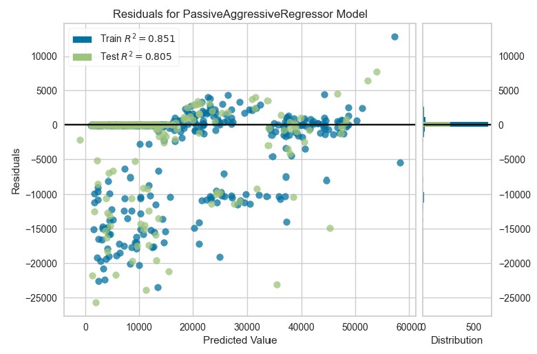
plot_model(par, plot="feature")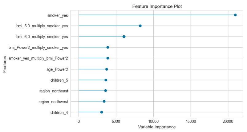
plot_model(par, plot = "error")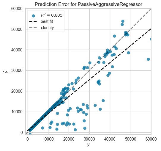
Blended Model
blender=blend_models(estimator_list=[tuned_ridge, lr, gbr, par])read.delim("texttable9.txt", sep = "\t") %>%as_tibble() %>%
gt() %>% tab_header(title = md("**Blended Model**")) %>%
gt_highlight_rows(rows = 11, font_weight = "normal")| Blended Model | ||||||
| Fold | MAE | MSE | RMSE | R2 | RMSLE | MAPE |
|---|---|---|---|---|---|---|
| 0 | 2408.0842 | 17302756 | 4159.658 | 0.8898 | 0.3869 | 0.2535 |
| 1 | 1863.4308 | 9320452 | 3052.941 | 0.9507 | 0.2753 | 0.2229 |
| 2 | 2282.9336 | 14762622 | 3842.216 | 0.8857 | 0.3599 | 0.2565 |
| 3 | 2654.2865 | 25483338 | 5048.102 | 0.7803 | 0.4712 | 0.2441 |
| 4 | 2829.9945 | 31288042 | 5593.572 | 0.8020 | 0.4538 | 0.2101 |
| 5 | 2481.5104 | 20045336 | 4477.202 | 0.8606 | 0.4005 | 0.2650 |
| 6 | 2564.7835 | 19534698 | 4419.807 | 0.8926 | 0.3474 | 0.2399 |
| 7 | 2478.1730 | 23479704 | 4845.586 | 0.7804 | 0.4929 | 0.2646 |
| 8 | 2064.9262 | 12575007 | 3546.126 | 0.9379 | 0.3530 | 0.2771 |
| 9 | 2410.9463 | 29548765 | 5435.878 | 0.7402 | 0.4522 | 0.1934 |
| Mean | 2403.9069 | 20334072 | 4442.109 | 0.8520 | 0.3993 | 0.2427 |
| Std | 265.2138 | 6810031 | 775.720 | 0.0683 | 0.0645 | 0.0252 |
plot_model(blender, plot="residuals")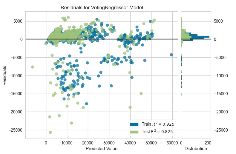
Save Blended Model
save_model(blender, model_name="pycaret_prod_example")Application Deployment
For this example, the app has been hosted on streamlit.io. Here is the link to the app.
The application can also be run locally using the Anaconda Prompt by moving to the folder where app.py lives and typing streamlit run app.py.