Process Mining
How is it different than traditional process mapping?
What is Process Mining?

Process mining is a relatively new discipline being used in enterprises to help them more accurately map and understand their processes. Once an organization accurately understands its’ processes, it can get a better insight into its overall functioning and then can proceed to improve and automate those processes. Process mining automatically generates process models with frequencies and performance measures (and more).
Process mining techniques allow for extracting information from event logs. For example, the audit trails of a workflow management system or the transaction logs of an enterprise resource planning system can be used to discover models describing processes, organizations, and products. Moreover, it is possible to use process mining to monitor deviations.
Process mining is a data science discipline that is often overlooked. What a shame. All businesses are driven by process - how is it possible that data science has overlooked this rich opportunity for operation improvement?
Garner estimates the overall market of process mining to approach around $1 Billion.
Process Mining vs Data Mining
Process mining is very different from basic data mining techniques. Although both process mining and data mining start from data, data mining techniques are typically not process-centric and do not focus on event data. Process mining combines process models and event data in various novel ways. As a result, it can find out what people and organizations really do. For example, process models can be automatically discovered from event data. Compliance can be checked by confronting models with event data. Bottlenecks can be uncovered by replaying timed events on discovered or normative models. Hence, process mining can be used to identify and understand bottlenecks, inefficiencies, deviations, and risks.
End-to-end process models and concurrency are essential for process mining. Moreover, topics such as process discovery, conformance checking, and bottleneck analysis are not addressed by traditional data mining techniques and tools.
Process mining bridges the gap between traditional model-based process analysis (e.g., simulation and other business process management techniques) and data-centric analysis techniques such as machine learning and data mining.
Some people consider process mining to be part of the broader data mining discipline This is just fine: it is merely a matter of definition. However, note that traditional text books on data mining do not consider processes. Questions related to performance (e.g., bottlenecks in processes) and compliance (e.g., quantifying and diagnosing deviations from some normative model) are not addressed at all. Moreover, none of the traditional data mining tools support process mining techniques in a satisfactory manner.
Data mining (in the narrow sense) and process mining are complementary approaches that can strengthen each other. Process models (once discovered and aligned with the event log) provide the basis for valuable data mining questions.
How is it different than traditional methods of Process Mapping?
Organizations have been using numerous process improvement methods and tools for many decades. Process mining tools allow organizations to chart out their processes based on the state of the actual data stored in their ERP, CRM, or other information systems. This allows organizations to accurately depict the functional state of the organization rather than relying on assumptions or speculation. So, while in traditional process mapping approaches it’s possible to miss various steps and activities when mapping a given process, the data-driven approach ensures that the process is mapped accurately. This then leads organizations to get better and intelligent insights, which they can then use to improve or automate their processes.
Benefits of Process Mining
Here are some of the key benefits of employing process mining tools and techniques in organizations.
- The data-driven approach allows for an accurate mapping of an organization’s business processes.
- Accurate mapping of an organization’s processes allows organizations to remove waste, make processes leaner, identify areas of high-cost, etc., and subsequently take steps to improve those areas. Using process mining tools, organizations, therefore, can better improve their customer interactions, improve customer journeys, and streamline back-end business processes.
- The data-driven approach allows for subsequent automation of the processes and also the application of AI (Artificial Intelligence), ML (Machine Learning), and RPA (Robotic Process Automation) techniques to automate the organization’s processes.
- As contemporary process mining tools are based on friendly and advanced graphical user interfaces, they allow a quick understanding of the organization’s processes while identifying multiple process improvement ideas.
Typical Steps in Process Mining
Here are some of the typical steps that are used in Process Mining.
- Identify the sources of data that the given business process touches.
- Configure the process mining tools to use this data (also referred to as an event log) before it runs to map the given business process.
- Map the business process from start to finish showing all the steps, systems, people, and data used in the process.
- Process mining tools can then help identify areas in the business process that may be impacting the speed and agility of the process. The enhanced and sophisticated user interface of process mining tools allows for better visualization of the process flow, potential areas of bottlenecks, and more.
- Based on real data, the process morning tools can identify areas which can be automated used RPA or other AI/ML techniques.
- Introduce new KPIs or improve the existing ones throughout the process improvement exercise. 7.The holistic view of the process can allow organizations to predict all outcomes of the process. Accordingly, they can fine-tune the process until they get it right.
Process Mining with R
One of the reasons I love R is there are packages to speed the delivery of solutions. In this case, bupaR is the tool of choice. bupaR is an open-source, integrated suite of R-packages for the handling and analysis of business process data. bupaR provides support for different stages in process analysis, such as importing and preprocessing event data, calculating descriptive statistics, process visualization and conformance checking.
bupaR provides training opportunities:
The bupaR Masterclass consist of 10 Module of 2 hours, organized over a period of 5 weeks.
- Module 1: Introduction to Process Mining
- Module 2: Process data in R
- Module 3: Control-flow analysis
- Module 4: Performance & organization
- Module 5: Event log building
- Module 6: Advanced process analytics I
- Module 7: Advanced process analytics II
- Module 8: Conformance Checking
- Module 9: Automated Process discovery
- Module 10: Process prediction
I believe I delve deepr into all the features bupaR provides before considering this formal training.
Data
Data for this project is from the BPI Challenge 2017. This is a contest held by the organizers of the International Workshop on Business Process Intelligence (BPIC).
The data pertains to a loan application process of a Dutch financial institute. The data contains all applications filed trough an online system in 2016 and their subsequent events until February 1st 2017.
# load BPI Challenge 2017 data set ####
#data <- read_csv('loanapplicationfile.csv', locale = locale(date_names = 'en', encoding = 'ISO-8859-1'))
data <- read_csv('loanapplicationfile.csv', show_col_types = FALSE)

data <- data %>% rename(start = starttimestamp, complete = endtimestamp)

data <- data %>% select(-c(Start_Timestamp, Complete_Timestamp))

# remove blanks from var names
names(data) <- str_replace_all(names(data), c(" " = "_" , "," = "" ))

glimpse(data)
Rows: 400,000
Columns: 22
$ Case_ID <chr> "Application_652823628", "Application_6528236…
$ Activity <chr> "A_Create Application", "A_Submitted", "A_Con…
$ Resource <chr> "User_1", "User_1", "User_1", "User_17", "Use…
$ Variant <chr> "Variant 2", "Variant 2", "Variant 2", "Varia…
$ Variant_index <dbl> 2, 2, 2, 2, 2, 2, 2, 2, 2, 2, 2, 2, 2, 2, 2, …
$ `(case)_ApplicationType` <chr> "New credit", "New credit", "New credit", "Ne…
$ `(case)_LoanGoal` <chr> "Existing loan takeover", "Existing loan take…
$ `(case)_RequestedAmount` <dbl> 20000, 20000, 20000, 20000, 20000, 20000, 200…
$ Accepted <lgl> NA, NA, NA, NA, NA, TRUE, NA, NA, NA, NA, NA,…
$ Action <chr> "Created", "statechange", "statechange", "Obt…
$ CreditScore <dbl> NA, NA, NA, NA, NA, 979, NA, NA, NA, NA, NA, …
$ EventID <chr> "Application_652823628", "ApplState_158205199…
$ EventOrigin <chr> "Application", "Application", "Application", …
$ FirstWithdrawalAmount <dbl> NA, NA, NA, NA, NA, 20000, NA, NA, NA, NA, NA…
$ MonthlyCost <dbl> NA, NA, NA, NA, NA, 498, NA, NA, NA, NA, NA, …
$ NumberOfTerms <dbl> NA, NA, NA, NA, NA, 44, NA, NA, NA, NA, NA, N…
$ OfferID <chr> NA, NA, NA, NA, NA, NA, "Offer_148581083", "O…
$ OfferedAmount <dbl> NA, NA, NA, NA, NA, 20000, NA, NA, NA, NA, NA…
$ Selected <lgl> NA, NA, NA, NA, NA, TRUE, NA, NA, NA, NA, NA,…
$ `lifecycle:transition` <chr> "complete", "complete", "complete", "start", …
$ start <dttm> 2016-01-01 09:51:15, 2016-01-01 09:51:15, 20…
$ complete <dttm> 2016-01-01 09:51:15, 2016-01-01 09:51:15, 20…In the BPI 2017 dataset, a process always starts from an activity labelled as A_Create Application and ends at activities labelled as A_Pending, A_Denied or A_Cancelled.
- A_Pending - All documents have been received and the assessment is positive.
- A_Denied - The application doesn’t satisfy the acceptance criteria. Hence, it is cancelled by the bank.
- A_Cancelled - The application is cancelled if applicant does not get back to the bank after an offer was sent out.
In addition to the above activities there is one more activity known as O_Create Offer which contains the data required for prediction of the outcome of the process. This is useful for machine learning and prediction. (This is not pursued in this document - yet.)
Clean Data
Remove activities where EventOrigin = Workflow.
data <- data %>% filter(EventOrigin != "Workflow")
data <- data %>% select(-c(Variant, Variant_index, `lifecycle:transition`, OfferID, FirstWithdrawalAmount, MonthlyCost,
                           NumberOfTerms, OfferedAmount))
To make things simpler, break the data into 2 pieces: Application Process and Offer Process.
data_Application <- data %>% filter(substr(Activity, 1, 1) == "A")
data_Offer <- data %>% filter(substr(Activity, 1, 1) == "O")

glimpse(data_Application)
Rows: 170,188
Columns: 14
$ Case_ID <chr> "Application_652823628", "Application_6528236…
$ Activity <chr> "A_Create Application", "A_Submitted", "A_Con…
$ Resource <chr> "User_1", "User_1", "User_1", "User_52", "Use…
$ `(case)_ApplicationType` <chr> "New credit", "New credit", "New credit", "Ne…
$ `(case)_LoanGoal` <chr> "Existing loan takeover", "Existing loan take…
$ `(case)_RequestedAmount` <dbl> 20000, 20000, 20000, 20000, 20000, 20000, 200…
$ Accepted <lgl> NA, NA, NA, NA, NA, NA, NA, NA, NA, NA, NA, N…
$ Action <chr> "Created", "statechange", "statechange", "sta…
$ CreditScore <dbl> NA, NA, NA, NA, NA, NA, NA, NA, NA, NA, NA, N…
$ EventID <chr> "Application_652823628", "ApplState_158205199…
$ EventOrigin <chr> "Application", "Application", "Application", …
$ Selected <lgl> NA, NA, NA, NA, NA, NA, NA, NA, NA, NA, NA, N…
$ start <dttm> 2016-01-01 09:51:15, 2016-01-01 09:51:15, 20…
$ complete <dttm> 2016-01-01 09:51:15, 2016-01-01 09:51:15, 20…rm(data)Data Processing for Process Mining
Some terminology:
- Case: The subject of your process, e.g. a customer, an order, a patient.
- Activity: A step in your process, e.g. receive order, sent payment, perform MRI SCAN, etc.
- Activity instance: The execution of a specific step for a specific case.
- Event: A registration connected to an activity instance, characterized by a single timestamp. E.g. the start of Perform MRI SCAN for Patient X.
- Resource: A person or machine that is related to the execution of (part of) an activity instance. E.g. the radiologist in charge of our MRI SCAN.
- Lifecycle status: An indication of the status of an activity instance connect to an event. Typical values are start, complete. Other possible values are schedule, suspend, resume, etc.
- Trace: A sequence of activities. The activity instances that belong to a case will result to a specific trace when ordered by the time each instance occurred.
eventlog vs activitylog
bupaR currently supports two different kinds of log formats, both of which are an extension on R dataframes:
eventlog: Event logs are created from dataframes in which each row represents a single event. This means that it has a single timestamp. activitylog: Activity logs are created from dataframes in which each row represents a single activity instances. This means it can has multiple timestamps, stored in different columns.
The data there are 2 timestamps. This suggests the data supports activitylog analysis. A summary is provided after the creation on the activity log. It provides useful information, particularly:
- How many events are in the data
- The number of cases
- How many different process paths exist in the data
my_activities_A <- activitylog(data_Application,
                      case_id = 'Case_ID',
                      activity_id = 'Activity',
                      resource_id = 'Resource',
                      timestamps = c('start', 'complete'))
my_activities_A %>% summary
Number of events: 340376
Number of cases: 22509
Number of traces: 77
Number of distinct activities: 10
Average trace length: 15
Start eventlog: 2016-01-01 09:51:15
End eventlog: 2017-01-26 09:11:10 Case_ID Activity Resource
Length:170188 Length:170188 Length:170188
Class :character Class :character Class :character
Mode :character Mode :character Mode :character
(case)_ApplicationType (case)_LoanGoal (case)_RequestedAmount
Length:170188 Length:170188 Min. : 0
Class :character Class :character 1st Qu.: 6000
Mode :character Mode :character Median : 12000
Mean : 15811
3rd Qu.: 20000
Max. :450000
Accepted Action CreditScore EventID
Mode:logical Length:170188 Min. : NA Length:170188
NA's:170188 Class :character 1st Qu.: NA Class :character
Mode :character Median : NA Mode :character
Mean :NaN
3rd Qu.: NA
Max. : NA
NA's :170188
EventOrigin Selected start
Length:170188 Mode:logical Min. :2016-01-01 09:51:15.00
Class :character NA's:170188 1st Qu.:2016-03-21 08:14:34.00
Mode :character Median :2016-06-07 16:17:41.00
Mean :2016-05-29 01:05:47.69
3rd Qu.:2016-08-03 14:55:42.75
Max. :2017-01-26 09:11:10.00
complete .order
Min. :2016-01-01 09:51:15.00 Min. : 1
1st Qu.:2016-03-21 08:14:34.00 1st Qu.: 42548
Median :2016-06-07 16:17:41.00 Median : 85094
Mean :2016-05-29 01:05:47.69 Mean : 85094
3rd Qu.:2016-08-03 14:55:42.75 3rd Qu.:127641
Max. :2017-01-26 09:11:10.00 Max. :170188
Explore the Activity Data
Review the activities in the data and how frequently they are represented:
my_activities_A %>% activities# A tibble: 10 × 3
Activity absolute_frequency relative_frequency
<chr> <int> <dbl>
1 A_Validating 27476 0.161
2 A_Accepted 22509 0.132
3 A_Concept 22509 0.132
4 A_Create Application 22509 0.132
5 A_Complete 22415 0.132
6 A_Incomplete 15699 0.0922
7 A_Submitted 14562 0.0856
8 A_Pending 12363 0.0726
9 A_Cancelled 7544 0.0443
10 A_Denied 2602 0.0153Plot the activities. The plot suggests that there is a loop in the process since A_Validating has more occurrences than A_Create_Application.
my_activities_A %>% activity_frequency(level = "activity") %>% plot()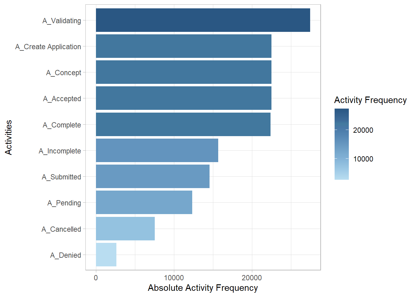
Review the 10 resources most frequently used in the process. User1 is involved nearly 28% of the time!
my_activities_A %>% resource_frequency('resource') %>% head(10)# A tibble: 10 × 3
Resource absolute relative
<chr> <int> <dbl>
1 User_1 46997 0.276
2 User_116 3225 0.0189
3 User_29 2964 0.0174
4 User_27 2651 0.0156
5 User_118 2549 0.0150
6 User_10 2511 0.0148
7 User_113 2475 0.0145
8 User_49 2427 0.0143
9 User_117 2411 0.0142
10 User_30 2312 0.0136# my_activities_A %>% filter_resource_frequency(perc = 0.90) %>% resources()bupar provides convenience by trimming cases so you can focus on pieces of a process that has specific interest:
my_activities_A %>%
    filter_trim(start_activities = "A_Accepted", end_activities =  c("A_Cancelled","A_Denied")) %>%
    process_map(type = performance())
In addition to focusing on specific parts of a process, bupar simplifies the analysis of specific timeframes:
my_activities_A %>%
  filter_time_period(interval = ymd(c(201601001, 20170201)), filter_method = "trim") %>%
  filter_trim(start_activities = "A_Accepted", end_activities =  c("A_Cancelled","A_Denied")) %>%
  process_map(type = performance())
Warning: 1 failed to parse.Explore Throughput & Processing Times:
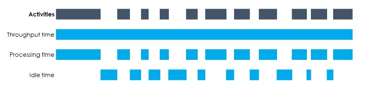
Three different time metrics can be computed:
- throughput time: the time between the very first event of the case and the very last
- processing time: the sum of the duration of all activity instances
- idle time: the time when no activity instance is active
The duration of an activity instance is the time between the first and the last event related to that activity instance. In case several activity instances within a case overlap, processing time for that overlap will be counted twice.
my_activities_A %>% throughput_time("log") %>% plot()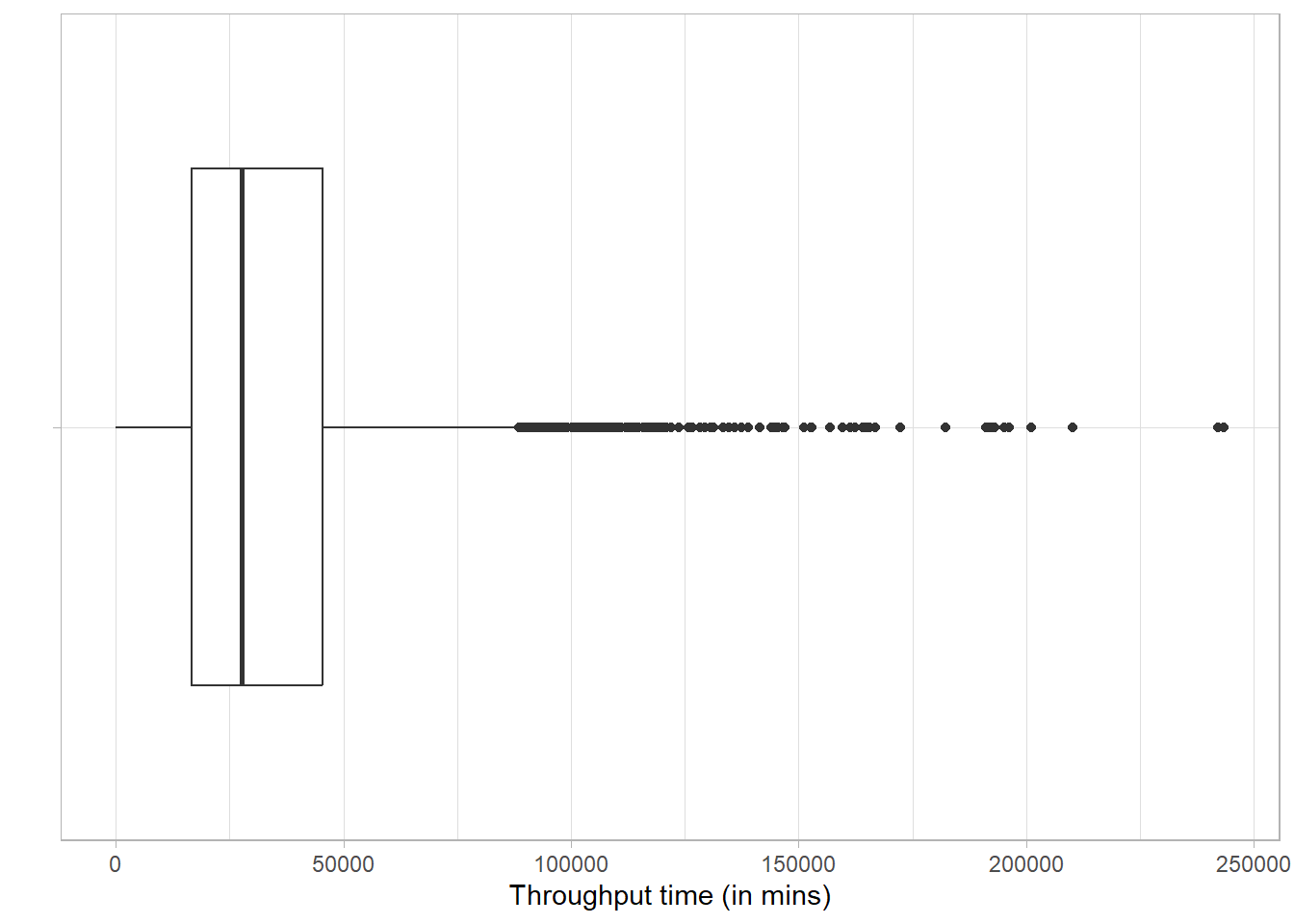
Note: The data used so far contains start and complete times that are the same value for each step in a given case:
data_Application %>% filter(Case_ID =="Application_652823628") %>% select(start, complete)# A tibble: 9 × 2
start complete
<dttm> <dttm>
1 2016-01-01 09:51:15 2016-01-01 09:51:15
2 2016-01-01 09:51:15 2016-01-01 09:51:15
3 2016-01-01 09:52:36 2016-01-01 09:52:36
4 2016-01-02 11:23:04 2016-01-02 11:23:04
5 2016-01-02 11:30:28 2016-01-02 11:30:28
6 2016-01-13 13:10:55 2016-01-13 13:10:55
7 2016-01-14 09:16:20 2016-01-14 09:16:20
8 2016-01-14 13:39:51 2016-01-14 13:39:51
9 2016-01-14 15:49:11 2016-01-14 15:49:11Therefore, the concept of processing time or idle time does not make sense. This is not a data problem, it simply reflects that the activities are performed electronically in this dataset - it does not capture the individual resource effort a specific activity requires. Therefore, to serve as an example for processing time and idle time, another dataset will be used (patient data) to illustrate these bupaR features.
patient_workflow <- eventdataR::patients
glimpse(patient_workflow)
Rows: 5,442
Columns: 7
$ handling <fct> Registration, Registration, Registration, Registrati…
$ patient <chr> "1", "2", "3", "4", "5", "6", "7", "8", "9", "10", "…
$ employee <fct> r1, r1, r1, r1, r1, r1, r1, r1, r1, r1, r1, r1, r1, …
$ handling_id <chr> "1", "2", "3", "4", "5", "6", "7", "8", "9", "10", "…
$ registration_type <fct> start, start, start, start, start, start, start, sta…
$ time <dttm> 2017-01-02 11:41:53, 2017-01-02 11:41:53, 2017-01-0…
$ .order <int> 1, 2, 3, 4, 5, 6, 7, 8, 9, 10, 11, 12, 13, 14, 15, 1…The processing time can be computed at the levels log, trace, case, activity and resource-activity. It can only be calculated when there are both start and end timestamps available for activity instances.
patient_workflow %>% processing_time("activity") %>% plot()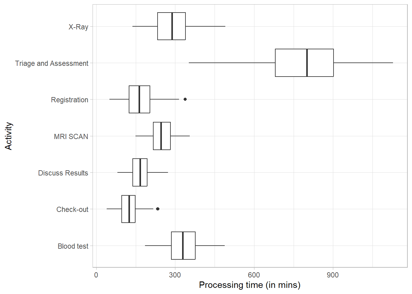
The idle time is the time that there is no activity in a case or for a resource. It can only be calculated when there are both start and end timestamps available for activity instances. It can be computed at the levels trace, resource, case and log, and using different time units.
patient_workflow %>%
    idle_time("resource", units = "days") %>%  plot()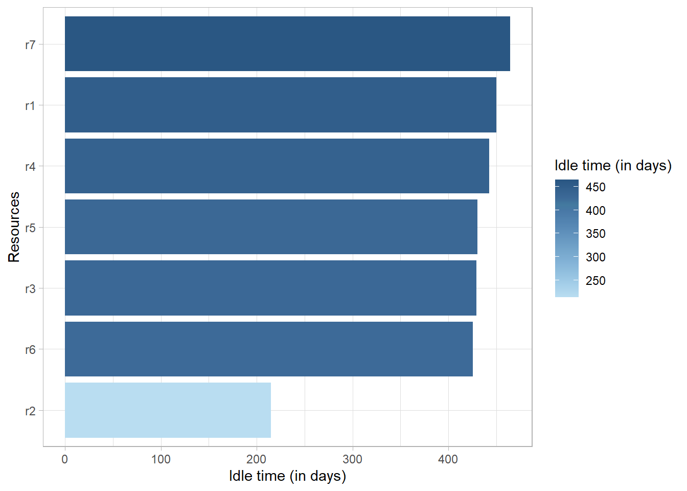
Process Maps
process_map automagically creates a process map of an event log.
my_activities_A %>% process_map(render = T) Rather than displaying absolute values, frequencies can be shown instead:
my_activities_A %>% process_map(type = frequency("relative"), render = T) The frequency value displayed can be one of the following
- absolute frequency: The absolute number of activity instances and flows
- absolute_case frequency: The absolute number of cases behind each activity and flow
- relative frequency:
- The relative number of instances per activity
- The relative outgoing flows for each activity
- relative_case frequency: The relative number of cases per activity and flow
The process map can also provide performance data so durations (process and idle times) can be evaluated.
my_activities_A %>% process_map(type_nodes = frequency("relative_case"), type_edges = performance(mean, "hours"))Process Maps - Animated!
To animate process maps, event logs are required. What has been used is activity log data. From the bupar website:
Currently both eventlog and activitylog are supported by the packages bupaR, edeaR and processmapR. The daqapo package only supports activitylog, while all other packages only support eventlog. While the goal is to extend support for both to all packages, you can in the meanwhile always convert the format of your log using the functions to_eventlog() and to_activitylog().↩︎
Below I have truncated that data to reduce animate_process runtime.
user_list <- paste0("User_", 1:20)

my_activities_A_2 <- my_activities_A %>% filter(Resource %in% user_list) %>%
  filter_time_period(interval = ymd(c(20161001, 20170201)), filter_method = "trim")

my_events <- to_eventlog(my_activities_A_2)

animate_process(my_events, jitter = 10, legend = "color", duration = 120,
                mapping = token_aes(color = token_scale("Resource", scale = "ordinal",
                                                        range = RColorBrewer::brewer.pal(7, "Paired"))))
Precedence Diagrams
A precendence diagrams is a two-dimensional matrix showing the flows between activities. It can be contain different type values, by adjusting the type argument.
- Absolute frequency of flows
- Relative frequency of flows
- Relative frequency of flows, for each antecendent
- Given antecendent A, it is followed x% of the time by Consequent B
- Relative frequency of flows, for each consequent
- Given consequent B, it is preceded x% of the time by Antecedent A
Note: Event log format required.
p1 <- precedence_matrix(my_events) %>% plot()
p2 <- precedence_matrix(my_events, type = "relative") %>% plot()

p1 / p2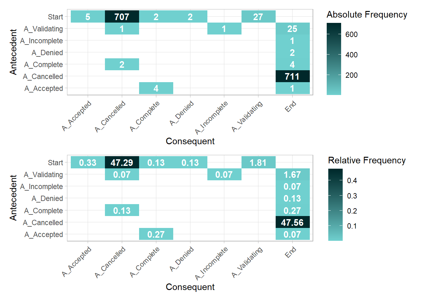
p3 <- precedence_matrix(my_events, type = "relative-antecedent") %>% plot()
p4 <- precedence_matrix(my_events, type = "relative-consequent") %>% plot()

p3 / p4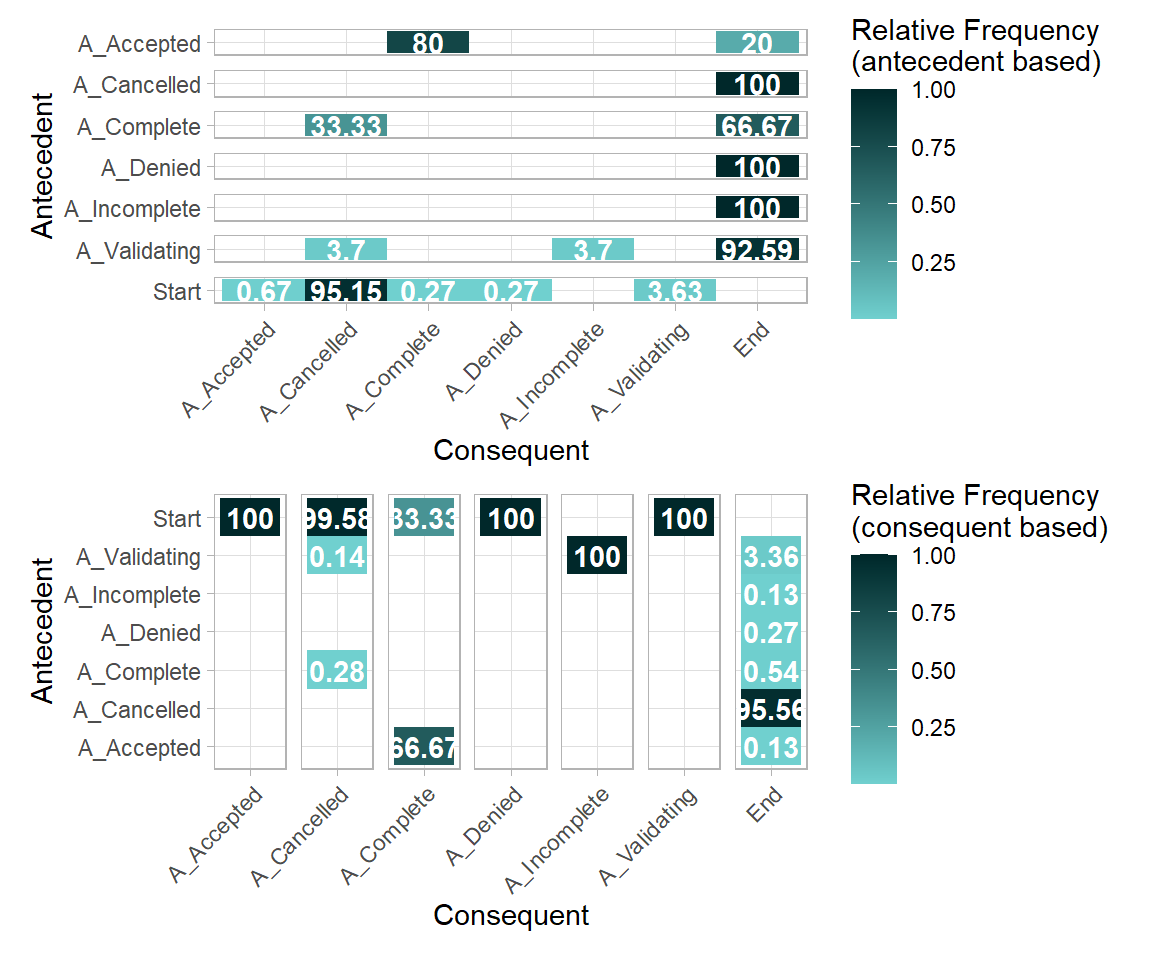
Trace Explorer
Different activity sequences in the event log can be visualized with trace_explorer. It can be used to explore frequent as well as infrequent traces. The coverage argument specifies how much of the log you want to explore. By default it is set at 0.2, meaning that it will show the most (in)frequency traces covering 20% of the event log.
Below, the top 50% of the sequences are displayed.
my_activities_A %>% trace_explorer(coverage = 0.5)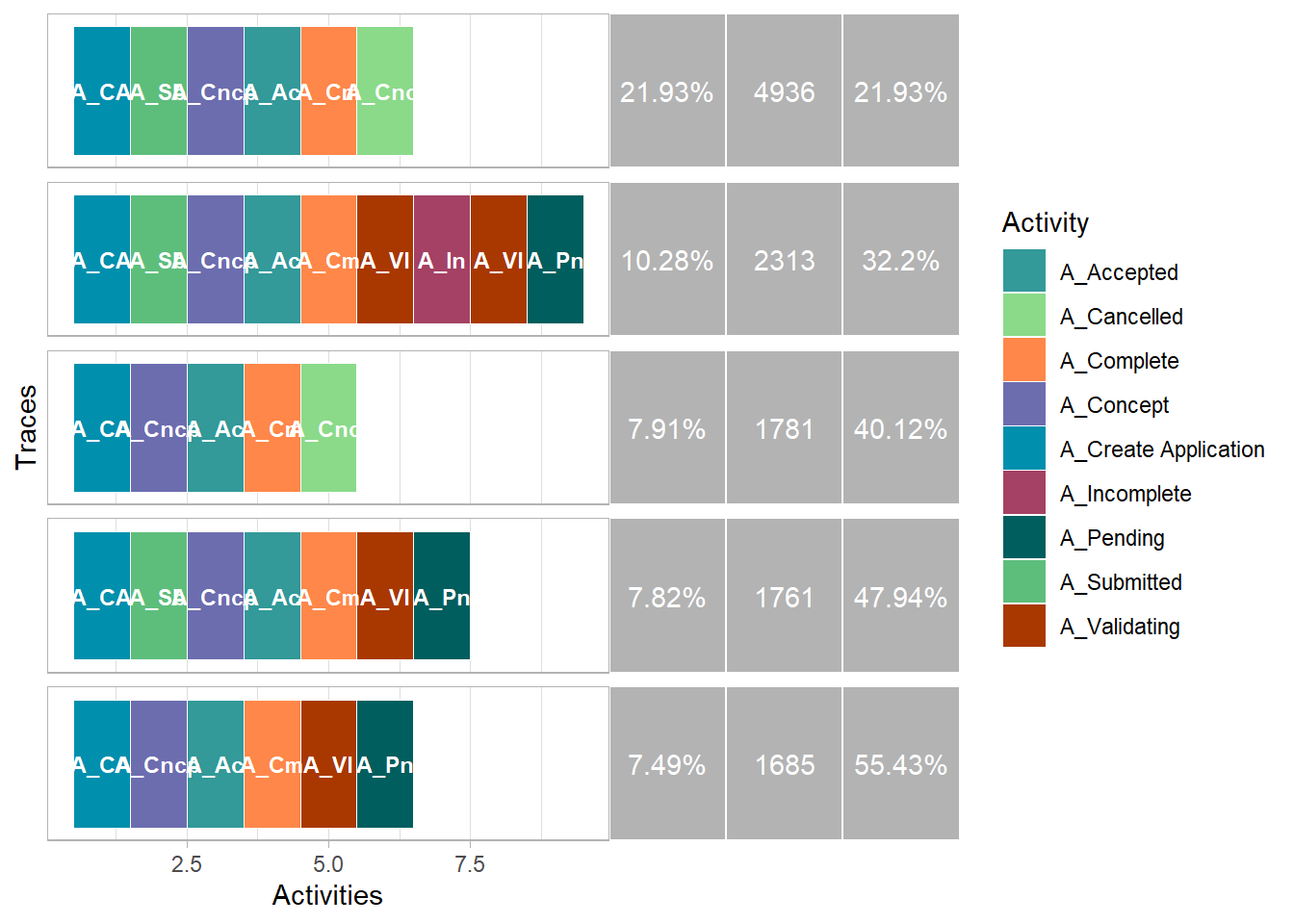
Dotted Plots
A dotted chart is a graph in which each activity instance is displayed with a point. The x-axis references to the time aspect, while the y-axis refers to cases. (The y axis can display information other than just cases (example: Resources). The dotted chart function has 3 arguments
- x: Either absolute (absolute time on x-axis) or relative (time difference since start case on x-axis)
- y: The ordering of the cases along the y-axis: by start, end, or duration.
- color: The attribute used to color the activity instances. Defaults to the activity type.
my_events %>% dotted_chart(color = "Resource")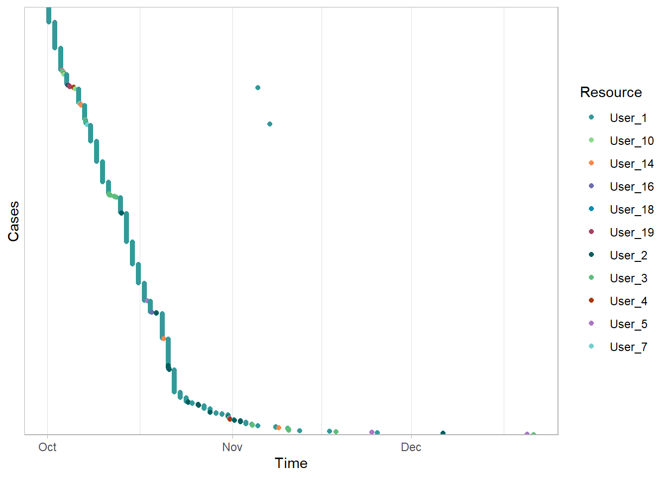
The data used in the plot serves as a poor example. Below is something more typical.
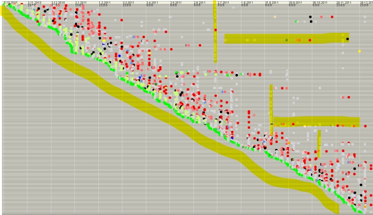 Note: - The incoming cases are steady. The line from the upper left to lower right is straight. - There are some activities performed in batches. Note the vertically highlighted activities. - Some cases take much longer that most. Note the horizontal cases highlighted.
These plots are very useful!
Resource Mapping
my_activities_A_2 %>%
  filter_activity_frequency(percentage = .1) %>% # show only most frequent resources
  filter_trace_frequency(percentage = .8) %>%    # show only the most frequent traces
  resource_map(render = T)
Miscellaneous Process Mining Techniques
bupar provides a wealth of other functions. If interested, take a look.
Filtering
# process map where one activity was at least once present in Oct 2016 ####
my_activities_A_2 %>%
  filter_time_period(interval = c(ymd(20161001), end_point = ymd(20161031)),
                     filter_method = 'start') %>%
  filter_activity_presence(activities = c('A_Cancelled')) %>%
  filter_activity_frequency(percentage = 1.0) %>% # show only most frequent activities
  filter_trace_frequency(percentage = .80) %>%    # show only the most frequent traces
  process_map(render = T)
Throughput
# Conditional Process Analysis ####
my_activities_A %>%
  filter_activity_frequency(percentage = 1.0) %>% # show only most frequent activities
  filter_trace_frequency(percentage = .80) %>%    # show only the most frequent traces
  throughput_time('log', units = 'hours')
# A tibble: 1 × 8
min q1 median mean q3 max st_dev iqr
<drtn> <drtn> <drtn> <drtn> <drtn> <drtn> <dbl> <drtn>
1 0.06 hours 269 hours 464 hours 523 hours 759 hours 3252 hours 293. 490 hourstmpData <- my_activities_A %>%
filter_activity_frequency(percentage = 1.0) %>% # show only most frequent activities
filter_trace_frequency(percentage = .80) %>% # show only the most frequent traces
throughput_time('case', units = 'hours')
tmpData <- as_tibble(tmpData)
bind_rows(tmpData %>% slice_max(throughput_time, n = 5, with_ties = F) %>% mutate(tier = "Max"),
tmpData %>% slice_min(throughput_time, n = 5, with_ties = F) %>% mutate(tier = "Min"))# A tibble: 10 × 3
Case_ID throughput_time tier
<chr> <drtn> <chr>
1 Application_983392205 3251.71 hours Max
2 Application_1499090661 2752.52 hours Max
3 Application_1171453988 2265.59 hours Max
4 Application_1108271369 2244.45 hours Max
5 Application_544368785 2013.24 hours Max
6 Application_522241789 0.06 hours Min
7 Application_1115683200 0.11 hours Min
8 Application_573813116 0.11 hours Min
9 Application_2072748824 0.12 hours Min
10 Application_748474109 0.13 hours Min my_activities_A %>%
filter_activity_frequency(percentage = 1.0) %>% # show only most frequent activities
filter_trace_frequency(percentage = .80) %>% # show only the most frequent traces
group_by(`(case)_ApplicationType`) %>%
throughput_time('log', units = 'hours')# A tibble: 2 × 9
`(case)_ApplicationType` min q1 median mean q3 max st_dev iqr
<chr> <drtn> <drt> <drtn> <drt> <drt> <drt> <dbl> <drt>
1 Limit raise 0.06 hou… 221 … 331 h… 406 … 554 … 1437… 241. 333 …
2 New credit 0.11 hou… 283 … 497 h… 538 … 762 … 3252… 295. 478 …my_activities_A %>%
filter_activity_frequency(percentage = 1.0) %>% # show only most frequent activities
filter_trace_frequency(percentage = .80) %>% # show only the most frequent traces
group_by(`(case)_LoanGoal`) %>%
throughput_time('log', units = 'hours')# A tibble: 14 × 9
`(case)_LoanGoal` min q1 median mean q3 max st_dev iqr
<chr> <drtn> <drt> <drtn> <drt> <drt> <drt> <dbl> <drt>
1 Boat 54.99 ho… 265 … 414 h… 504 … 747 … 1385… 281. 482 …
2 Business goal 233.01 ho… 329 … 748 h… 638 … 758 … 1245… 310. 430 …
3 Car 0.14 ho… 243 … 412 h… 500 … 759 … 1982… 290. 517 …
4 Caravan / Camper 56.25 ho… 219 … 331 h… 438 … 733 … 1629… 282. 514 …
5 Debt restructuring 731.85 ho… 732 … 732 h… 732 … 732 … 732… NA 0 …
6 Existing loan takeover 1.20 ho… 312 … 525 h… 565 … 764 … 2753… 299. 451 …
7 Extra spending limit 43.23 ho… 263 … 452 h… 505 … 756 … 1464… 266. 493 …
8 Home improvement 0.17 ho… 300 … 481 h… 536 … 760 … 1938… 283. 460 …
9 Motorcycle 57.84 ho… 239 … 404 h… 488 … 762 … 1338… 277. 522 …
10 Not speficied 0.59 ho… 326 … 636 h… 578 … 782 … 2244… 302. 457 …
11 Other, see explanation 0.51 ho… 283 … 476 h… 526 … 760 … 1723… 281. 477 …
12 Remaining debt home 0.62 ho… 339 … 673 h… 630 … 805 … 3252… 366. 466 …
13 Tax payments 51.40 ho… 287 … 419 h… 496 … 746 … 1220… 266. 459 …
14 Unknown 0.06 ho… 211 … 352 h… 437 … 735 … 2013… 286. 524 …Addendum
Before developing the code within this document, I completed a Coursera Course called Process Mining: Data Science in Action.
The course explains the key analysis techniques in process mining. You learn various process discovery algorithms. These can be used to automatically learn process models from raw event data. Various other process analysis techniques that use event data will be presented. Moreover, the course provides easy-to-use software, real-life data sets, and practical skills to directly apply the theory in a variety of application domains.
The course follows a book written by the author that also leads the Coursera Course. Process Mining: Data Science in Action 2nd Ed 2016
The course ignores R and Python solutions. But, it did introduce me to tools that might be of interest. Disco and ProM were briefly introduced. Other commercial solutions are also available:
- Perceptive Process Mining (before Futura Reflect and BPM|one) (Perceptive Software)
- ARIS Process Performance Manager (Software AG)
- QPR ProcessAnalyzer (QPR)
- Celonis Discovery (Celonis)
- Interstage Process Discovery (Fujitsu)
- Discovery Analyst (StereoLOGIC)
- XMAnalyzer (XMPro
Disco provides commercial solutions but does make a free edition that is limited to 100 events. This is a significant limitation but the application is very easy to use and is a great alternative to coding in R or Python for more casual business users. Highly recommended.
ProM is a free open source solution that is very powerful offering far more advanced features than Disco. However, it is much more complex and targeted to researchers and process engineers dedicated to the discipline. Training is available, something I may pursue.