Dog Breeds by Popularity
Introduction
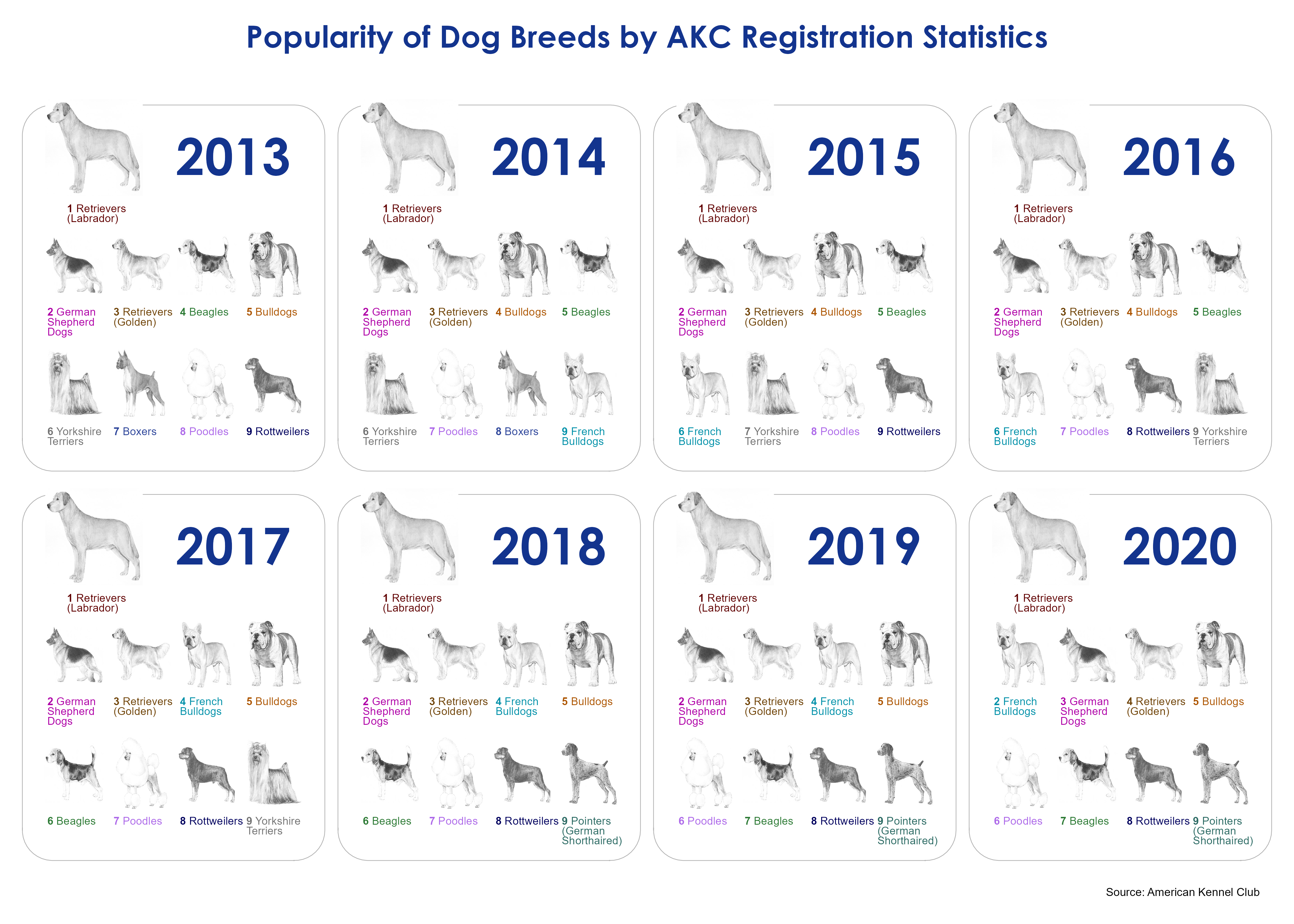
Each year, Americans purchase nearly 1 million purebred dogs, ranging from the 34-inch tall great dane to the 6-pound affenpinscher. These dogs are registered through the American Kennel Club (AKC), which categorizes and tallies up the totals of more than 150 breeds.
A dataset of these registrations going back 80 years —shows that Americans’ taste in dogs has dramatically changed over time.
# Must run first!
library(extrafont)
loadfonts(device = "win", quiet = TRUE) if(!require(easypackages)){install.packages("easypackages")}
library(easypackages)
packages("tidyverse", "ggimage", "magick", "ggtext","grid", "kableExtra", prompt = FALSE)Introduction
This is what we will create:
# out.width = "300px", echo = FALSE}
knitr::include_graphics("dogs.png")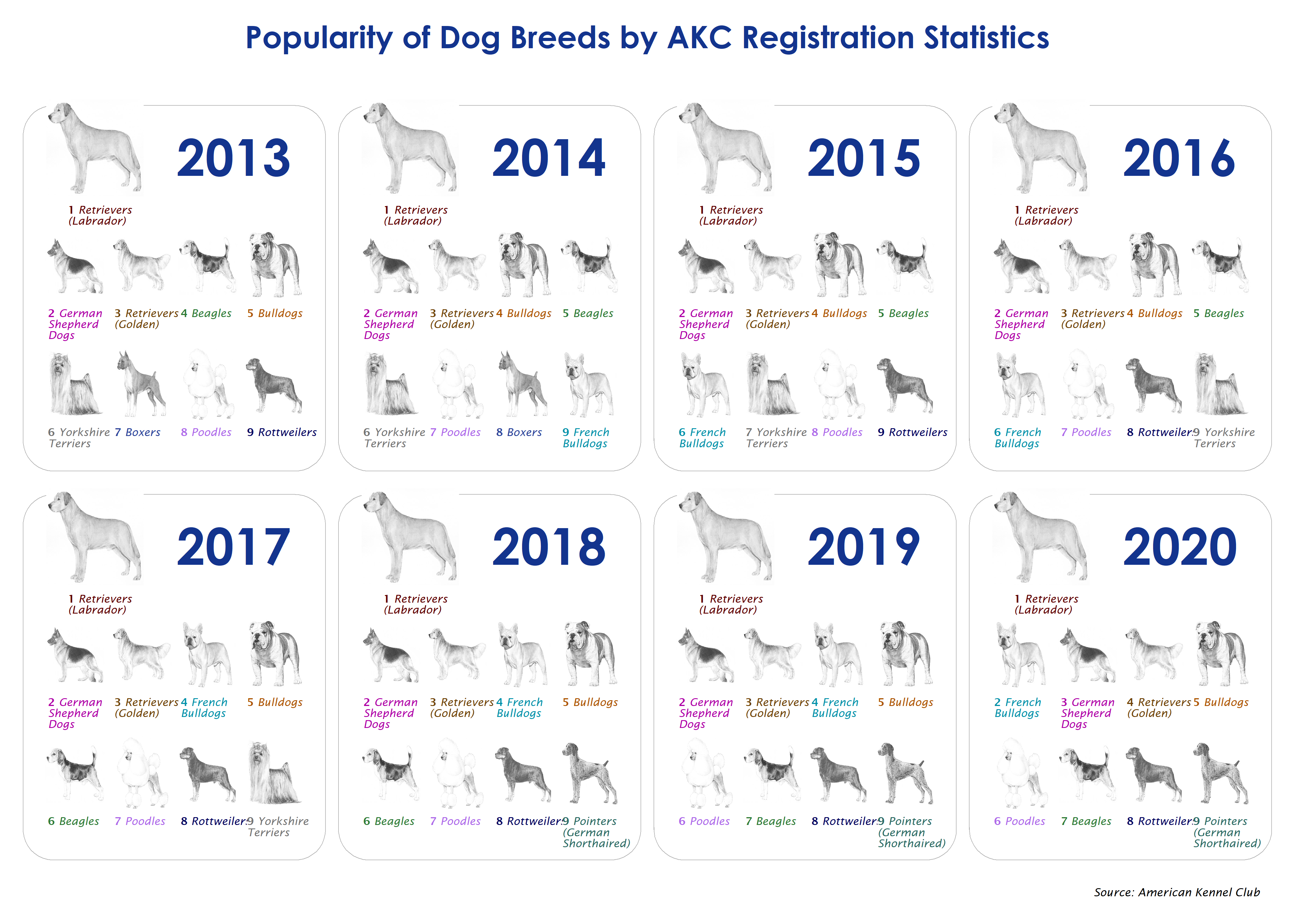
There are 9 dogs displayed for each of the 8 years. Each dog in each year panel needs to be precisely placed. (This is why x, y coordiantes are added to the dataframe created below.)
This is why significant design must be performed first - before any thought to start coding!
Libraries
extrafont- must be loaded first! This allow use of all installed TTF fonts.tidyverse- if you do not know this package, stop reading and take a basic R course!ggimage-ggimagesupports image files and graphic objects to be visualized inggplot2graphic system. Viginettemagick- The magick package provides a modern and simple toolkit for image processing in R.ggtext- Aggplot2extension that enables the rendering of complex formatted plot labels (titles, subtitles, facet labels, axis labels, etc.). Text boxes with automatic word wrap are also supported. Viginettegrid- grid is a low-level graphics system which provides a great deal of control and flexibility in the appearance and arrangement of graphical output.colorspace- The colorspace package provides a broad toolbox for selecting individual colors or color palettes, manipulating these colors, and employing them in various kinds of visualizations.
Data
Raw Data
breed_rank <- readr::read_csv('https://raw.githubusercontent.com/rfordatascience/tidytuesday/master/data/2022/2022-02-01/breed_rank.csv')
breed_rank %>% head(10) %>% kbl() %>% kable_paper("striped", full_width = F)| Breed | 2013 Rank | 2014 Rank | 2015 Rank | 2016 Rank | 2017 Rank | 2018 Rank | 2019 Rank | 2020 Rank | links | Image |
|---|---|---|---|---|---|---|---|---|---|---|
| Retrievers (Labrador) | 1 | 1 | 1 | 1 | 1 | 1 | 1 | 1 | https://www.akc.org/dog-breeds/labrador-retriever/ | https://www.akc.org/wp-content/uploads/2017/11/Labrador-Retriever-illustration.jpg |
| French Bulldogs | 11 | 9 | 6 | 6 | 4 | 4 | 4 | 2 | https://www.akc.org/dog-breeds/french-bulldog/ | https://www.akc.org/wp-content/uploads/2017/11/French-Bulldog-Illo-2.jpg |
| German Shepherd Dogs | 2 | 2 | 2 | 2 | 2 | 2 | 2 | 3 | https://www.akc.org/dog-breeds/german-shepherd-dog/ | https://www.akc.org/wp-content/uploads/2017/11/German-Shepherd-Dog-Illo-2.jpg |
| Retrievers (Golden) | 3 | 3 | 3 | 3 | 3 | 3 | 3 | 4 | https://www.akc.org/dog-breeds/golden-retriever/ | https://www.akc.org/wp-content/uploads/2017/11/Golden-Retriever-Illo-2.jpg |
| Bulldogs | 5 | 4 | 4 | 4 | 5 | 5 | 5 | 5 | https://www.akc.org/dog-breeds/bulldog/ | https://www.akc.org/wp-content/uploads/2017/11/Bulldog-Illo-2.jpg |
| Poodles | 8 | 7 | 8 | 7 | 7 | 7 | 6 | 6 | https://www.akc.org/dog-breeds/poodle-standard/ | https://www.akc.org/wp-content/uploads/2017/11/Standard-Poodle-illustration.jpg |
| Beagles | 4 | 5 | 5 | 5 | 6 | 6 | 7 | 7 | https://www.akc.org/dog-breeds/beagle/ | https://www.akc.org/wp-content/uploads/2017/11/Beagle-Illo-2.jpg |
| Rottweilers | 9 | 10 | 9 | 8 | 8 | 8 | 8 | 8 | https://www.akc.org/dog-breeds/rottweiler/ | https://www.akc.org/wp-content/uploads/2017/11/Rottweiler-Illo-2.jpg |
| Pointers (German Shorthaired) | 13 | 12 | 11 | 11 | 10 | 9 | 9 | 9 | https://www.akc.org/dog-breeds/german-shorthaired-pointer/ | https://www.akc.org/wp-content/uploads/2017/11/German-Shorthaired-Pointer-Illo-2.jpg |
| Dachshunds | 10 | 11 | 13 | 13 | 13 | 12 | 11 | 10 | https://www.akc.org/dog-breeds/dachshund/ | https://www.akc.org/wp-content/uploads/2017/11/Dachshund-Illo-2.jpg |
Data Wrangling
breed_rank %>% janitor::clean_names() %>%
head(10) %>% kbl() %>% kable_paper("striped", full_width = T)| breed | x2013_rank | x2014_rank | x2015_rank | x2016_rank | x2017_rank | x2018_rank | x2019_rank | x2020_rank | links | image |
|---|---|---|---|---|---|---|---|---|---|---|
| Retrievers (Labrador) | 1 | 1 | 1 | 1 | 1 | 1 | 1 | 1 | https://www.akc.org/dog-breeds/labrador-retriever/ | https://www.akc.org/wp-content/uploads/2017/11/Labrador-Retriever-illustration.jpg |
| French Bulldogs | 11 | 9 | 6 | 6 | 4 | 4 | 4 | 2 | https://www.akc.org/dog-breeds/french-bulldog/ | https://www.akc.org/wp-content/uploads/2017/11/French-Bulldog-Illo-2.jpg |
| German Shepherd Dogs | 2 | 2 | 2 | 2 | 2 | 2 | 2 | 3 | https://www.akc.org/dog-breeds/german-shepherd-dog/ | https://www.akc.org/wp-content/uploads/2017/11/German-Shepherd-Dog-Illo-2.jpg |
| Retrievers (Golden) | 3 | 3 | 3 | 3 | 3 | 3 | 3 | 4 | https://www.akc.org/dog-breeds/golden-retriever/ | https://www.akc.org/wp-content/uploads/2017/11/Golden-Retriever-Illo-2.jpg |
| Bulldogs | 5 | 4 | 4 | 4 | 5 | 5 | 5 | 5 | https://www.akc.org/dog-breeds/bulldog/ | https://www.akc.org/wp-content/uploads/2017/11/Bulldog-Illo-2.jpg |
| Poodles | 8 | 7 | 8 | 7 | 7 | 7 | 6 | 6 | https://www.akc.org/dog-breeds/poodle-standard/ | https://www.akc.org/wp-content/uploads/2017/11/Standard-Poodle-illustration.jpg |
| Beagles | 4 | 5 | 5 | 5 | 6 | 6 | 7 | 7 | https://www.akc.org/dog-breeds/beagle/ | https://www.akc.org/wp-content/uploads/2017/11/Beagle-Illo-2.jpg |
| Rottweilers | 9 | 10 | 9 | 8 | 8 | 8 | 8 | 8 | https://www.akc.org/dog-breeds/rottweiler/ | https://www.akc.org/wp-content/uploads/2017/11/Rottweiler-Illo-2.jpg |
| Pointers (German Shorthaired) | 13 | 12 | 11 | 11 | 10 | 9 | 9 | 9 | https://www.akc.org/dog-breeds/german-shorthaired-pointer/ | https://www.akc.org/wp-content/uploads/2017/11/German-Shorthaired-Pointer-Illo-2.jpg |
| Dachshunds | 10 | 11 | 13 | 13 | 13 | 12 | 11 | 10 | https://www.akc.org/dog-breeds/dachshund/ | https://www.akc.org/wp-content/uploads/2017/11/Dachshund-Illo-2.jpg |
breed_rank %>% janitor::clean_names() %>% pivot_longer(x2013_rank:x2020_rank, names_to = "year", values_to = "rank") %>%
head(10) %>% kbl() %>% kable_paper("striped", full_width = F)| breed | links | image | year | rank |
|---|---|---|---|---|
| Retrievers (Labrador) | https://www.akc.org/dog-breeds/labrador-retriever/ | https://www.akc.org/wp-content/uploads/2017/11/Labrador-Retriever-illustration.jpg | x2013_rank | 1 |
| Retrievers (Labrador) | https://www.akc.org/dog-breeds/labrador-retriever/ | https://www.akc.org/wp-content/uploads/2017/11/Labrador-Retriever-illustration.jpg | x2014_rank | 1 |
| Retrievers (Labrador) | https://www.akc.org/dog-breeds/labrador-retriever/ | https://www.akc.org/wp-content/uploads/2017/11/Labrador-Retriever-illustration.jpg | x2015_rank | 1 |
| Retrievers (Labrador) | https://www.akc.org/dog-breeds/labrador-retriever/ | https://www.akc.org/wp-content/uploads/2017/11/Labrador-Retriever-illustration.jpg | x2016_rank | 1 |
| Retrievers (Labrador) | https://www.akc.org/dog-breeds/labrador-retriever/ | https://www.akc.org/wp-content/uploads/2017/11/Labrador-Retriever-illustration.jpg | x2017_rank | 1 |
| Retrievers (Labrador) | https://www.akc.org/dog-breeds/labrador-retriever/ | https://www.akc.org/wp-content/uploads/2017/11/Labrador-Retriever-illustration.jpg | x2018_rank | 1 |
| Retrievers (Labrador) | https://www.akc.org/dog-breeds/labrador-retriever/ | https://www.akc.org/wp-content/uploads/2017/11/Labrador-Retriever-illustration.jpg | x2019_rank | 1 |
| Retrievers (Labrador) | https://www.akc.org/dog-breeds/labrador-retriever/ | https://www.akc.org/wp-content/uploads/2017/11/Labrador-Retriever-illustration.jpg | x2020_rank | 1 |
| French Bulldogs | https://www.akc.org/dog-breeds/french-bulldog/ | https://www.akc.org/wp-content/uploads/2017/11/French-Bulldog-Illo-2.jpg | x2013_rank | 11 |
| French Bulldogs | https://www.akc.org/dog-breeds/french-bulldog/ | https://www.akc.org/wp-content/uploads/2017/11/French-Bulldog-Illo-2.jpg | x2014_rank | 9 |
breed_rank %>% janitor::clean_names() %>% pivot_longer(x2013_rank:x2020_rank, names_to = "year", values_to = "rank") %>%

filter(rank < 10) %>% mutate(year = parse_number(year)) %>% group_by(year) %>% arrange(rank) %>%
head(10) %>% kbl() %>% kable_paper("striped", full_width = F)| breed | links | image | year | rank |
|---|---|---|---|---|
| Retrievers (Labrador) | https://www.akc.org/dog-breeds/labrador-retriever/ | https://www.akc.org/wp-content/uploads/2017/11/Labrador-Retriever-illustration.jpg | 2013 | 1 |
| Retrievers (Labrador) | https://www.akc.org/dog-breeds/labrador-retriever/ | https://www.akc.org/wp-content/uploads/2017/11/Labrador-Retriever-illustration.jpg | 2014 | 1 |
| Retrievers (Labrador) | https://www.akc.org/dog-breeds/labrador-retriever/ | https://www.akc.org/wp-content/uploads/2017/11/Labrador-Retriever-illustration.jpg | 2015 | 1 |
| Retrievers (Labrador) | https://www.akc.org/dog-breeds/labrador-retriever/ | https://www.akc.org/wp-content/uploads/2017/11/Labrador-Retriever-illustration.jpg | 2016 | 1 |
| Retrievers (Labrador) | https://www.akc.org/dog-breeds/labrador-retriever/ | https://www.akc.org/wp-content/uploads/2017/11/Labrador-Retriever-illustration.jpg | 2017 | 1 |
| Retrievers (Labrador) | https://www.akc.org/dog-breeds/labrador-retriever/ | https://www.akc.org/wp-content/uploads/2017/11/Labrador-Retriever-illustration.jpg | 2018 | 1 |
| Retrievers (Labrador) | https://www.akc.org/dog-breeds/labrador-retriever/ | https://www.akc.org/wp-content/uploads/2017/11/Labrador-Retriever-illustration.jpg | 2019 | 1 |
| Retrievers (Labrador) | https://www.akc.org/dog-breeds/labrador-retriever/ | https://www.akc.org/wp-content/uploads/2017/11/Labrador-Retriever-illustration.jpg | 2020 | 1 |
| French Bulldogs | https://www.akc.org/dog-breeds/french-bulldog/ | https://www.akc.org/wp-content/uploads/2017/11/French-Bulldog-Illo-2.jpg | 2020 | 2 |
| German Shepherd Dogs | https://www.akc.org/dog-breeds/german-shepherd-dog/ | https://www.akc.org/wp-content/uploads/2017/11/German-Shepherd-Dog-Illo-2.jpg | 2013 | 2 |
Grid Coordinates
Create x, y coordinates for organizing the plot. These values are used to place the dog breed image in each of the 8 year panels.
The dogs have been ranked and there are 1-9 ranks.
Develop x Coordinates:
- Start with a value of 0.75
- Repeat a sequence of values starting with 0.5 to 3
- The code automatically calculates values between 0.5 and 3 to create 4 evenly spaced values
- The sequence is repeated 2 times
x = c(0.75, rep(seq(0.5, 3, length.out = 4), 2))
x
[1] 0.750000 0.500000 1.333333 2.166667 3.000000 0.500000 1.333333 2.166667
[9] 3.000000Develop y Coordinates:
- start with a value of 3
- repeat the vlaues 1.5 and 0 four times
y = c(3, rep(c(1.5, 0), each = 4))
y
[1] 3.0 1.5 1.5 1.5 1.5 0.0 0.0 0.0 0.0tibble(x, y)# A tibble: 9 × 2
x y
<dbl> <dbl>
1 0.75 3
2 0.5 1.5
3 1.33 1.5
4 2.17 1.5
5 3 1.5
6 0.5 0
7 1.33 0
8 2.17 0
9 3 0 top_breeds <- breed_rank %>% janitor::clean_names() %>%
pivot_longer(x2013_rank:x2020_rank, names_to = "year", values_to = "rank") %>%
filter(rank < 10) %>% mutate(year = parse_number(year)) %>% group_by(year) %>% arrange(rank) %>%
mutate(x = c(0.75, rep(seq(0.5, 3, length.out = 4), 2)),
y = c(3, rep(c(1.5, 0), each = 4)))
top_breeds %>% head(10) %>% kbl() %>% kable_paper("striped", full_width = F)| breed | links | image | year | rank | x | y |
|---|---|---|---|---|---|---|
| Retrievers (Labrador) | https://www.akc.org/dog-breeds/labrador-retriever/ | https://www.akc.org/wp-content/uploads/2017/11/Labrador-Retriever-illustration.jpg | 2013 | 1 | 0.75 | 3.0 |
| Retrievers (Labrador) | https://www.akc.org/dog-breeds/labrador-retriever/ | https://www.akc.org/wp-content/uploads/2017/11/Labrador-Retriever-illustration.jpg | 2014 | 1 | 0.75 | 3.0 |
| Retrievers (Labrador) | https://www.akc.org/dog-breeds/labrador-retriever/ | https://www.akc.org/wp-content/uploads/2017/11/Labrador-Retriever-illustration.jpg | 2015 | 1 | 0.75 | 3.0 |
| Retrievers (Labrador) | https://www.akc.org/dog-breeds/labrador-retriever/ | https://www.akc.org/wp-content/uploads/2017/11/Labrador-Retriever-illustration.jpg | 2016 | 1 | 0.75 | 3.0 |
| Retrievers (Labrador) | https://www.akc.org/dog-breeds/labrador-retriever/ | https://www.akc.org/wp-content/uploads/2017/11/Labrador-Retriever-illustration.jpg | 2017 | 1 | 0.75 | 3.0 |
| Retrievers (Labrador) | https://www.akc.org/dog-breeds/labrador-retriever/ | https://www.akc.org/wp-content/uploads/2017/11/Labrador-Retriever-illustration.jpg | 2018 | 1 | 0.75 | 3.0 |
| Retrievers (Labrador) | https://www.akc.org/dog-breeds/labrador-retriever/ | https://www.akc.org/wp-content/uploads/2017/11/Labrador-Retriever-illustration.jpg | 2019 | 1 | 0.75 | 3.0 |
| Retrievers (Labrador) | https://www.akc.org/dog-breeds/labrador-retriever/ | https://www.akc.org/wp-content/uploads/2017/11/Labrador-Retriever-illustration.jpg | 2020 | 1 | 0.75 | 3.0 |
| French Bulldogs | https://www.akc.org/dog-breeds/french-bulldog/ | https://www.akc.org/wp-content/uploads/2017/11/French-Bulldog-Illo-2.jpg | 2020 | 2 | 0.50 | 1.5 |
| German Shepherd Dogs | https://www.akc.org/dog-breeds/german-shepherd-dog/ | https://www.akc.org/wp-content/uploads/2017/11/German-Shepherd-Dog-Illo-2.jpg | 2013 | 2 | 0.50 | 1.5 |
Design
Fonts
Importing fonts can be frustrating. This article solved my problem. Specifically:
library(extrafont)
library(remotes)
remotes::install_version("Rttf2pt1", version = "1.3.8")
extrafont::font_import()
This article is also valuable.
fonts() [1] "Agency FB" "Algerian"
[3] "Arial Black" "Arial"
[5] "Arial Narrow" "Arial Rounded MT Bold"
[7] "Bahnschrift" "Baskerville Old Face"
[9] "Bauhaus 93" "Bell MT"
[11] "Berlin Sans FB" "Berlin Sans FB Demi"
[13] "Bernard MT Condensed" "Blackadder ITC"
[15] "Bodoni MT" "Bodoni MT Black"
[17] "Bodoni MT Condensed" "Bodoni MT Poster Compressed"
[19] "Book Antiqua" "Bookman Old Style"
[21] "Bookshelf Symbol 7" "Bradley Hand ITC"
[23] "Britannic Bold" "Broadway"
[25] "Brush Script MT" "Calibri"
[27] "Calibri Light" "Californian FB"
[29] "Calisto MT" "Cambria"
[31] "Candara" "Candara Light"
[33] "Castellar" "Centaur"
[35] "Century" "Century Gothic"
[37] "Century Schoolbook" "Chiller"
[39] "Colonna MT" "Comic Sans MS"
[41] "Consolas" "Constantia"
[43] "Cooper Black" "Copperplate Gothic Bold"
[45] "Copperplate Gothic Light" "Corbel"
[47] "Corbel Light" "Courier New"
[49] "Curlz MT" "Dubai"
[51] "Dubai Light" "Dubai Medium"
[53] "DYMO Symbols" "Ebrima"
[55] "Edwardian Script ITC" "Elephant"
[57] "Engravers MT" "Eras Bold ITC"
[59] "Eras Demi ITC" "Eras Light ITC"
[61] "Eras Medium ITC" "Felix Titling"
[63] "Footlight MT Light" "Forte"
[65] "Franklin Gothic Book" "Franklin Gothic Demi"
[67] "Franklin Gothic Demi Cond" "Franklin Gothic Heavy"
[69] "Franklin Gothic Medium" "Franklin Gothic Medium Cond"
[71] "Freestyle Script" "French Script MT"
[73] "Gabriola" "Gadugi"
[75] "Garamond" "Georgia"
[77] "Gigi" "Gill Sans Ultra Bold"
[79] "Gill Sans Ultra Bold Condensed" "Gill Sans MT"
[81] "Gill Sans MT Condensed" "Gill Sans MT Ext Condensed Bold"
[83] "Gloucester MT Extra Condensed" "Goudy Old Style"
[85] "Goudy Stout" "Haettenschweiler"
[87] "Harlow Solid Italic" "Harrington"
[89] "High Tower Text" "HoloLens MDL2 Assets"
[91] "Impact" "Imprint MT Shadow"
[93] "Informal Roman" "Ink Free"
[95] "Javanese Text" "Jokerman"
[97] "Juice ITC" "Kristen ITC"
[99] "Kunstler Script" "Wide Latin"
[101] "Leelawadee UI" "Leelawadee UI Semilight"
[103] "Lucida Bright" "Lucida Calligraphy"
[105] "Lucida Console" "Lucida Fax"
[107] "Lucida Handwriting" "Lucida Sans"
[109] "Lucida Sans Typewriter" "Lucida Sans Unicode"
[111] "Magneto" "Maiandra GD"
[113] "Malgun Gothic" "Malgun Gothic Semilight"
[115] "Marlett" "Matura MT Script Capitals"
[117] "Microsoft Himalaya" "Microsoft Yi Baiti"
[119] "Microsoft New Tai Lue" "Microsoft PhagsPa"
[121] "Microsoft Sans Serif" "Microsoft Tai Le"
[123] "Mistral" "Modern No. 20"
[125] "Mongolian Baiti" "Monotype Corsiva"
[127] "MS Outlook" "MS Reference Sans Serif"
[129] "MS Reference Specialty" "MT Extra"
[131] "MV Boli" "Myanmar Text"
[133] "Niagara Engraved" "Niagara Solid"
[135] "Nirmala UI" "Nirmala UI Semilight"
[137] "OCR A Extended" "Old English Text MT"
[139] "Onyx" "Palace Script MT"
[141] "Palatino Linotype" "Papyrus"
[143] "Parchment" "Perpetua"
[145] "Perpetua Titling MT" "Playbill"
[147] "Poor Richard" "Pristina"
[149] "Rage Italic" "Ravie"
[151] "Rockwell" "Rockwell Condensed"
[153] "Rockwell Extra Bold" "Script MT Bold"
[155] "Segoe Fluent Icons" "Segoe MDL2 Assets"
[157] "Segoe Print" "Segoe Script"
[159] "Segoe UI" "Segoe UI Light"
[161] "Segoe UI Semibold" "Segoe UI Semilight"
[163] "Segoe UI Black" "Segoe UI Historic"
[165] "Segoe UI Symbol" "Segoe UI Variable"
[167] "Showcard Gothic" "SimSun-ExtB"
[169] "Sitka Text" "Snap ITC"
[171] "Stencil" "Sylfaen"
[173] "Symbol" "Tahoma"
[175] "Tempus Sans ITC" "Times New Roman"
[177] "Trebuchet MS" "Tw Cen MT"
[179] "Tw Cen MT Condensed" "Tw Cen MT Condensed Extra Bold"
[181] "Verdana" "Viner Hand ITC"
[183] "Vivaldi" "Vladimir Script"
[185] "Webdings" "Wingdings"
[187] "Wingdings 2" "Wingdings 3"
[189] "Outfit Thin" "Porpora"
[191] "Sans Serif Collection" "Sharpie" On Windows, view the here:
C:\Windows\Fonts
Here is a site where you can find similar fonts should you need one you do not have.
#f1 = "Porpora"
f1 = "Microsoft Sans Serif Regular"
#f2 = "Proxima Nova"
f2 = "Lucida Sans"
#f3 = "Futura"
f3 = "Century Gothic"font_add_google("")Colors
pal <- colorspace::darken(c("#3cb44b", "#4363d8", "#f58231", "#42d4f4", "#f032e6", "#469990", "#dcbeff", "#9A6324", "#800000", "#000075", "#a9a9a9", "#000000"), 0.3)Plotting
Create Grob
annotation_custom- Fromggplotis a special geom intended for use as static annotations that are the same in every panel. These annotations will not affect scales (i.e. the x and y axes will not grow to cover the range of thegrob, and thegrobwill not be modified by anyggplotsettings or mappings).grob- Fromgrid. Creating grid graphical objects, short (grobs).roundrectGrob- Fromgrid. Draw a single rectangle with rounded corners.gp- Graphical parameters to apply to thegrob.lwd- is line width. -gpar()is used to create a set of graphical parameter settings. It returns an object of classgpar. This is basically a list of name-value pairs.
geom_image- Fromggimage. Displays the image. controls placement, size and aspect ratio. Maintain aspect can be found here.geom_text- Fromggplot. Textgeomsare useful for labeling plots. They can be used by themselves as scatterplots or in combination with other geoms, for example, for labeling points or for annotating the height of bars.geom_text()adds only text to the plot.stat- The statistical transformation to use on the data for this layer, as a string.
g1 <- ggplot(top_breeds) +
  # Rounded rect
  annotation_custom(grob = grid::roundrectGrob(gp = gpar(col = "grey70", fill = NA, lwd = 0.75)),
                    xmin = -0.15, xmax = 3.65, ymin = -1.1, ymax = 3.5) +
  # No 1 image
  geom_image(data = top_breeds %>% filter(rank == 1), aes(x, y, image = image), size = 0.35, asp = 1.2) +
  # No 2-9 images
  geom_image(data = top_breeds %>% filter(rank > 1), aes(x, y, image = image), size = 0.22, asp = 1.2) +
  # Year
  geom_text(aes(2.5, 2.85, label = year), stat = "unique", family = f3, fontface = "bold", size = 14, color = "#13348E")
g1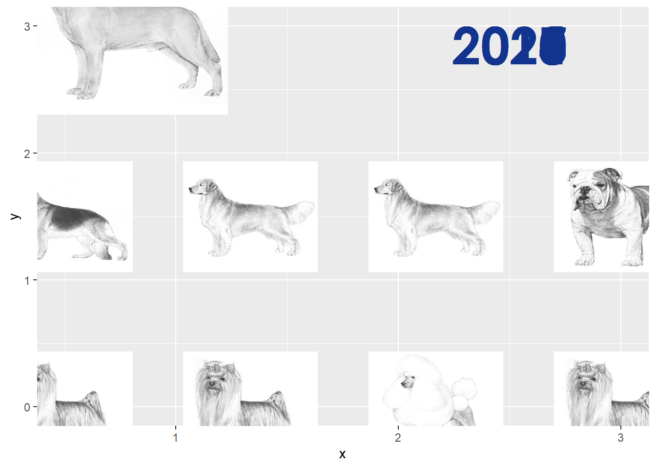
Rank and Breed Text
geom_textbox- Fromggtext. Draw boxes of defined width and height containing word-wrapped text.
g2 <- g1 + geom_textbox(aes(x + 0.1,
                            ifelse(rank == 1, y - 0.75, y - 0.55),
                            label = str_wrap(paste0("**", rank, "** ", breed), 15),
                            color = breed),
                        family = f2, size = 3, lineheight = 0.9, vjust = 1, width = 0.25,
                        box.padding = unit(0, "mm"), box.color = NA)
g2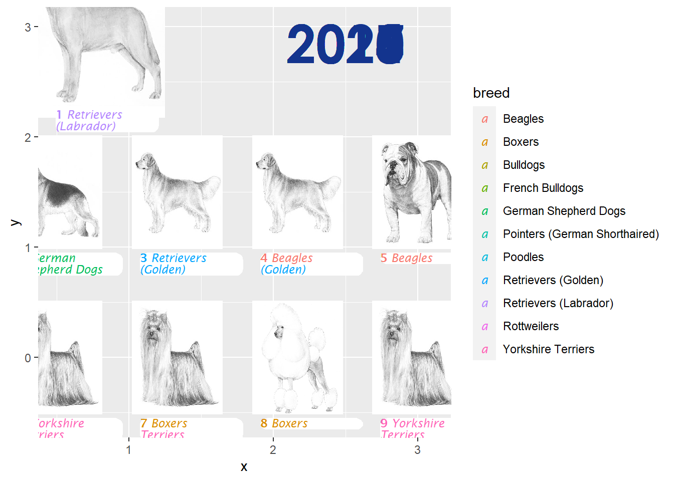
Coordinates & Text Additions
coord_fixed- A fixed scale coordinate system forces a specified ratio between the physical representation of data units on the axes. The ratio represents the number of units on the y-axis equivalent to one unit on the x-axis. The default, ratio = 1, ensures that one unit on the x-axis is the same length as one unit on the y-axis. Ratios higher than one make units on the y axis longer than units on the x-axis, and vice versa. Documentationexpand = FALSE- If TRUE, the default, adds a small expansion factor to the limits to ensure that data and axes don’t overlap. If FALSE, limits are taken exactly from the data orxlim/ylim.clip = "off"- Should drawing be clipped to the extent of the plot panel? A setting of “on” (the default) means yes, and a setting of “off” means no. In most cases, the default of “on” should not be changed, as settingclip = "off"can cause unexpected results. It allows drawing of data points anywhere on the plot, including in the plot margins. If limits are set viaxlimandylimand some data points fall outside those limits, then those data points may show up in places such as the axes, the legend, the plot title, or the plot margins.panel.spacing.x/panel.spacing.y- Adds more white space between the margins of each panel in the plot.element_text- Specifies the display of how non-data components of the plot are drawn.- element_blank(): draws nothing, and assigns no space
- element_rect(): borders and backgrounds
- element_line(): lines
- element_text(): text
margin(0, 0, 40, 0)/margin(90, 0, 0, 0)/margin(20, 20, 20, 20)- Used to specify the margins of elements.margin(t = 0, r = 0, b = 0, l = 0, unit = "pt")Remember this by thinking trouble.
g3 <- g2 + coord_fixed(xlim = c(0, 3.5), ylim = c(0, 3.5), expand = FALSE, clip = "off") +
  scale_color_manual(values = pal) +
  facet_wrap(vars(year), nrow = 2) +
  labs(title = ("Popularity of Dog Breeds by AKC Registration Statistics"),
       caption = "Source: American Kennel Club") +
  theme_void(base_family = f2) +
  theme(legend.position = "none",
        plot.background = element_rect(fill = "white", color = NA),
        strip.text = element_blank(),
        panel.spacing.x = unit(2, "lines"),
        panel.spacing.y = unit(6, "lines"),
        plot.title = element_text(size = 24, hjust = 0.5, family = f3, margin = margin(0, 0, 40, 0),
                                  face = "bold", color = "#13348E"),
        plot.caption = element_text(margin = margin(90, 0, 0, 0)),
        plot.margin = margin(20, 20, 20, 20))
g3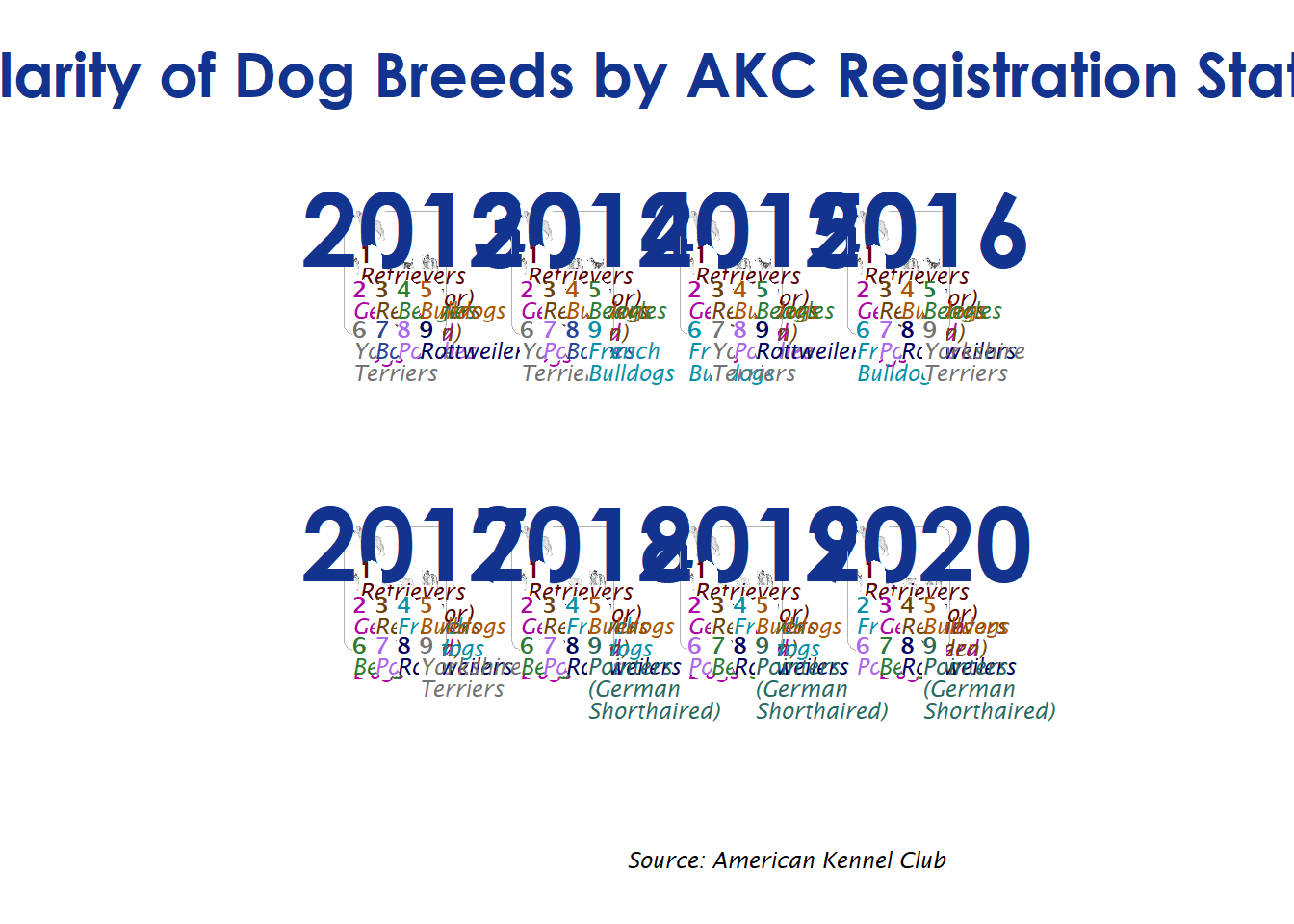
Save File
ggsave("Dog_Breeds.png", g3, width = 14, height = 10, units = "in", dpi = 320)Remember - plots do not always show-up properly within RStudio.
# out.width = "300px", echo = FALSE}
knitr::include_graphics("Dog_Breeds.png")